WARNING: This article may be obsolete
This post was published in 2022-10-11. Obviously, expired content is less useful to users if it has already pasted its expiration date.
 This article is categorized as "Garbage" . It should NEVER be appeared in your search engine's results.
Table of Contents
又一次记错了harmonic series和octave的关系
又一次记错了harmonic series和octave的关系,再次回顾:
🔗 [2021-12-31 - Truxton's blog] https://truxton2blog.com/2021-12-31/

离散傅里叶变换
公式(来源:奥本海姆《离散时间信号处理》P436~P437):
[mathjax-d]X[k]=\sum_{n=0}^{N-1}x[n]e^{-jk\frac{2\pi}{N}n}[/mathjax-d]以及
[mathjax-d]x[n]=\frac{1}{N}\sum_{k=0}^{N-1}X[k]e^{jk\frac{2\pi}{N}n}[/mathjax-d]奥本海姆《离散时间信号处理》P436~P437原公式(在符号用法上略有不同)
同时注意到系数[mathjax]\frac{1}{N}[/mathjax]的位置和奥本海姆《信号与系统》P135的不同(本质结果都是一样的)。
使用上面这个公式可以对应熟悉的bin frequency->frequency转换公式。
此外,奥本海姆的书上限定了带波浪线的[mathjax]\tilde{x}[n][/mathjax]是周期信号序列。但我们有的时候也可以“硬用”这个公式,因为有限序列是否周期截断是无从查证的,如果我们硬要说它是周期截断那也没有问题。所以:
如果[mathjax]x[n][/mathjax]是周期序列(对周期信号的周期截断),那么变换后的频谱是符合我们要求的。
如果[mathjax]x[n][/mathjax]不是周期序列(非周期截断,所以我们硬把[mathjax]N[/mathjax]当作它的周期),那么变换后的频谱存在能量泄漏。
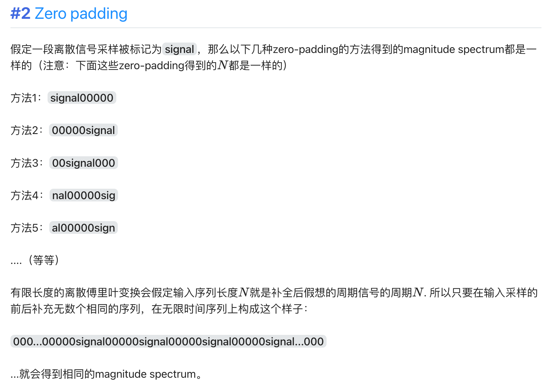
研究一下zero-padding问题
我对这篇文章里的zero-padding结论充满了疑惑和怀疑:
🔗 [ASPMA补充材料(2):(zero) padding, zero phase zero padding - Truxton's blog] https://truxton2blog.com/aspma-syllabus-review-supplement-2-zero-padding-zero-phase/#Zero_padding
现在应该差不多解决了。新结论如下:
参考过的资料:
🔗 [Zero-Phase Zero Padding] https://ccrma.stanford.edu/~jos/sasp/Zero_Phase_Zero_Padding.html
🔗 [fft - Merits of "Zero-Phase" Zero Padding - Signal Processing Stack Exchange] https://dsp.stackexchange.com/questions/18938/merits-of-zero-phase-zero-padding
继续学习傅里叶级数/傅里叶变换的一些性质
从2022-10-08继续,学习傅里叶级数/傅里叶变换的一些性质:
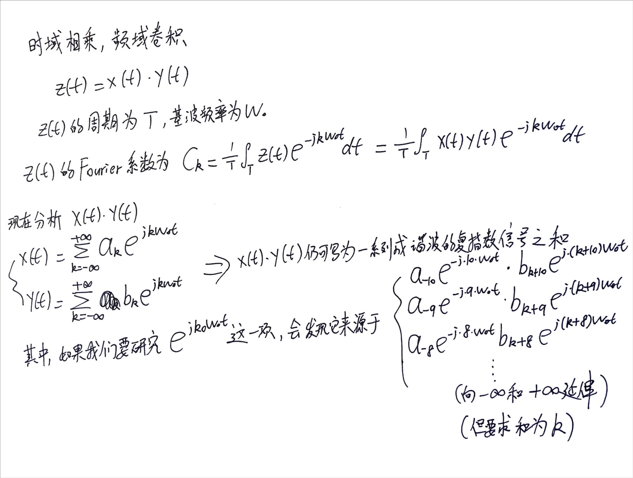
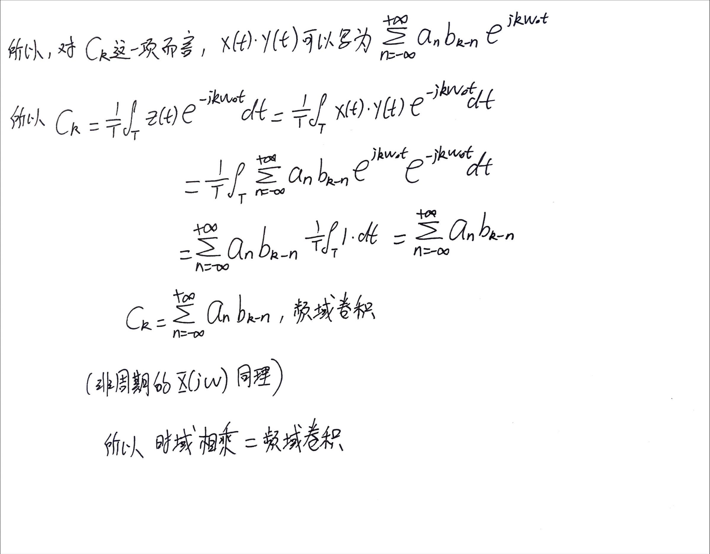
相乘性质
相乘性质
这部分内容应该是很重要的内容才对(和 卷积性质 互补),但暂时没有找到该部分内容在李琳山教授公开课里的对应视频。
这部分内容的证明方法1:
🔗 [如何证明连续时间傅里叶级数的相乘性质?_百度知道] https://zhidao.baidu.com/question/2058873342080339867.html
自己写的方法:
通过观看李琳山老师的视频从头开始复习一些性质
内容1
先放在一边,从这里开始从头复习:
🔗 [10信號與系統 Unit10 Continuous-time Fourier Transform(I)_哔哩哔哩_bilibili] https://www.bilibili.com/video/BV1dM4y1M7LK?p=10
看到不熟悉的内容就先记下来
BV1dM4y1M7LK p10 31:00左右
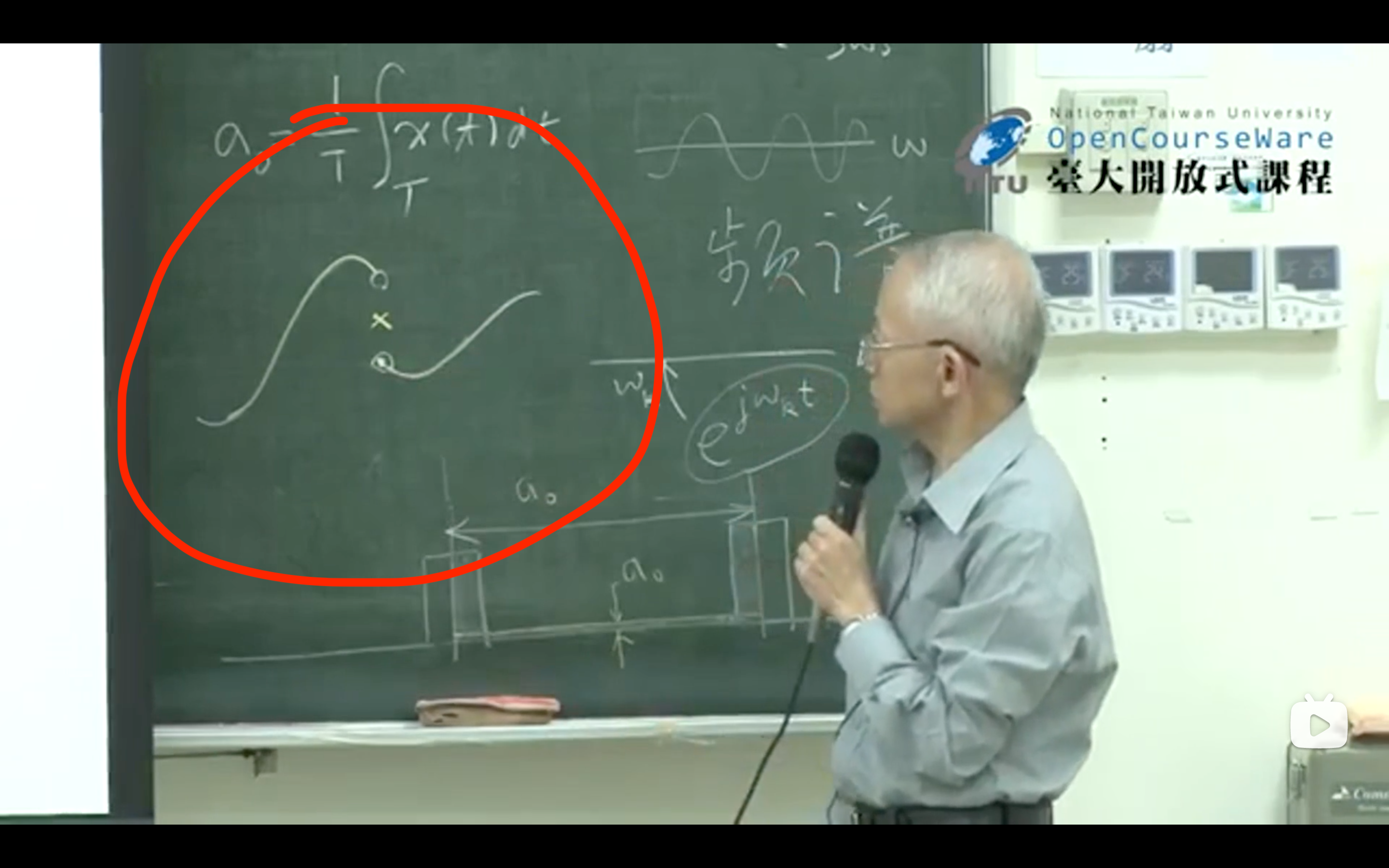
如果有红圈所示的信号[mathjax]x(t)[/mathjax],这个信号在某一时刻有一个不连续的“断点”(其余部分均为连续),那么对这个信号[mathjax]x(t)[/mathjax]做傅里叶变换,然后又做一次逆傅里叶变换得到[mathjax]x^{\prime}(t)[/mathjax],那么[mathjax]x^{\prime}(t)[/mathjax]还会是原来那个有断点的信号吗?
不是的。[mathjax]x^{\prime}(t)[/mathjax]会在原来的“断点”处取中间值,然后除了这个断点以外,其余部分均和原有信号[mathjax]x(t)[/mathjax]相同。
从BV1dM4y1M7LK p10 40:10左右开始讲述continous-time fourier transform properties
共轭/conjugate 性质
共轭/conjugate 性质
书P129
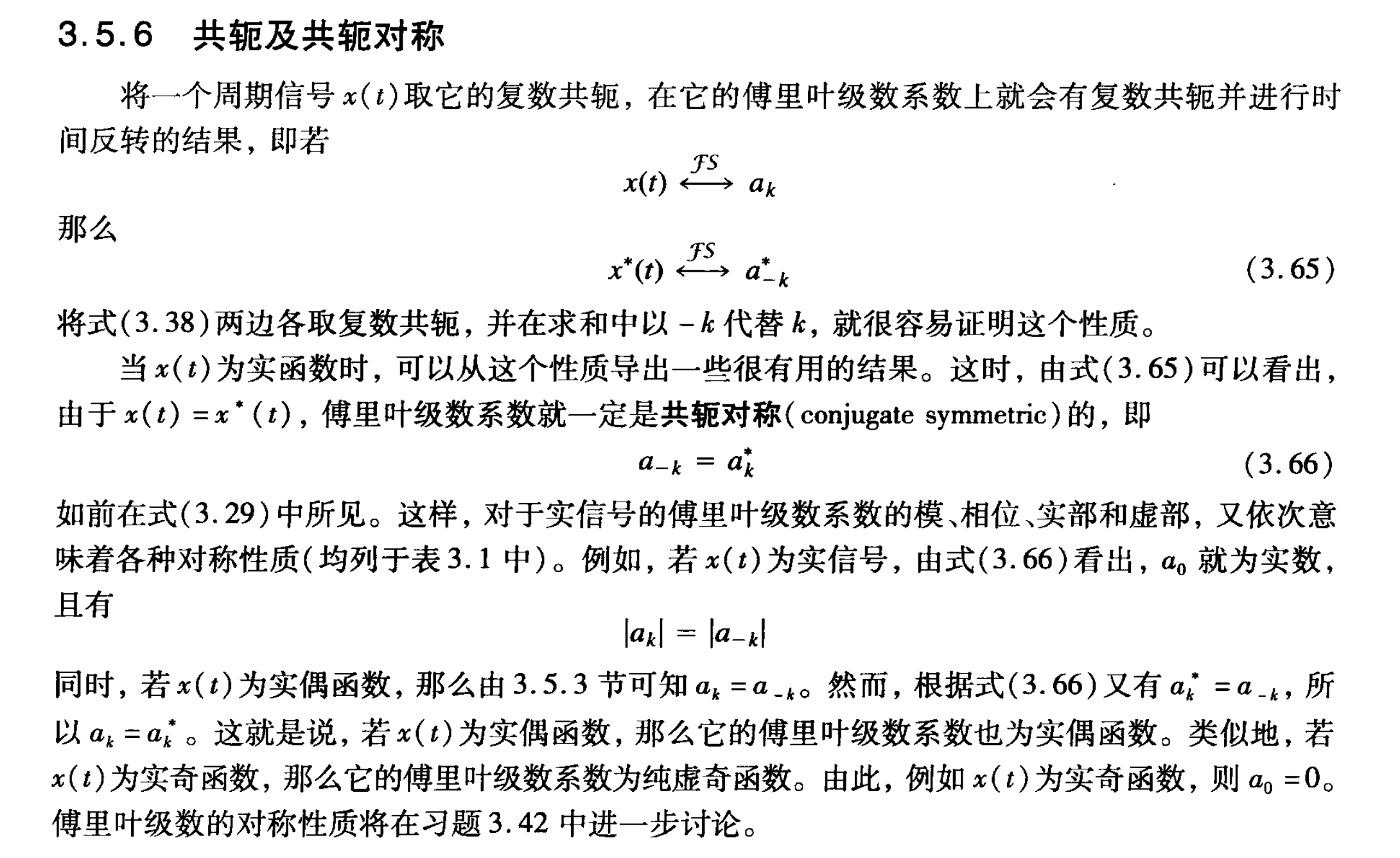
或者视频:BV1dM4y1M7LK p10 45:17左右
推导:(第二页纸有点混乱,但基本结果应该是对的)
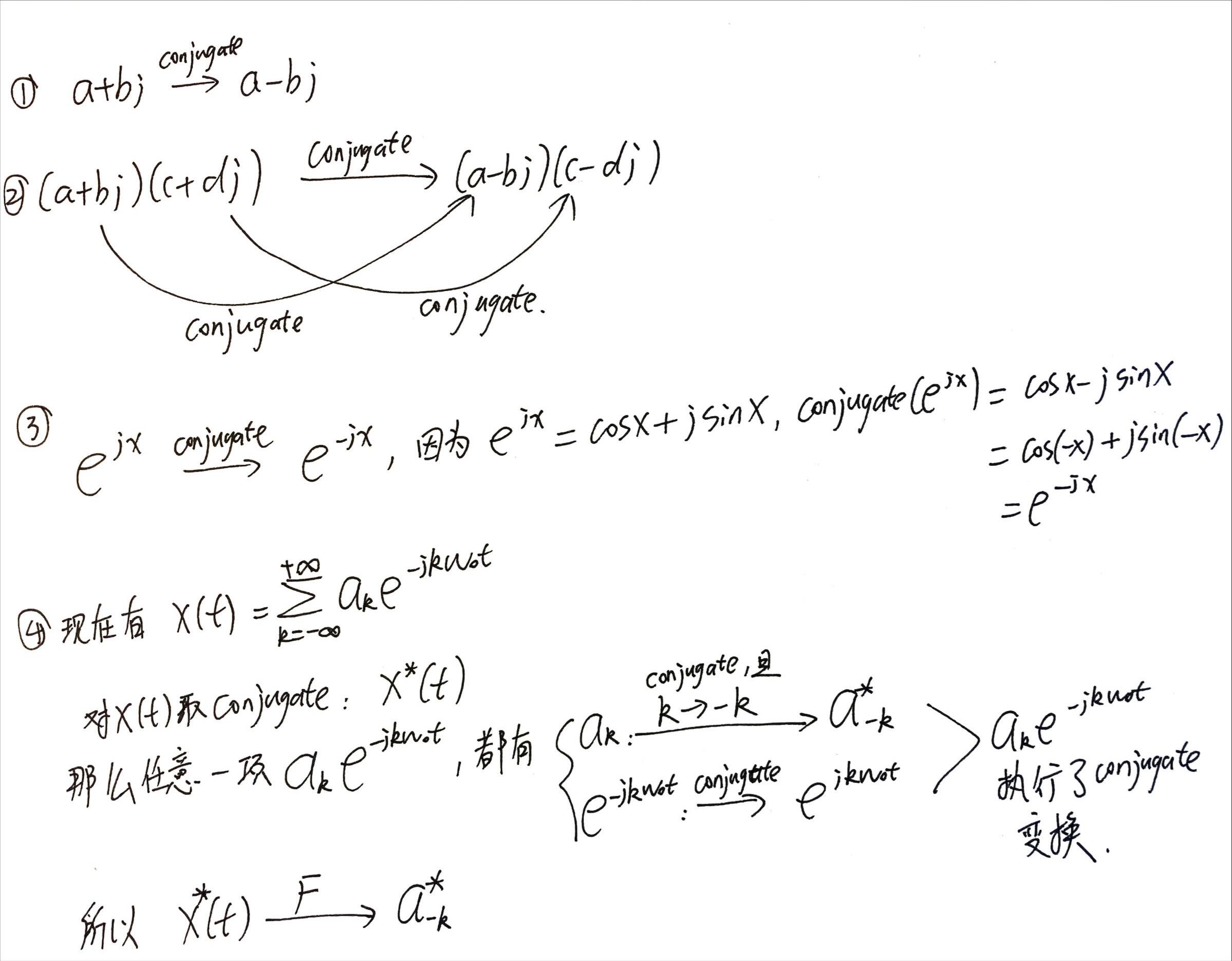
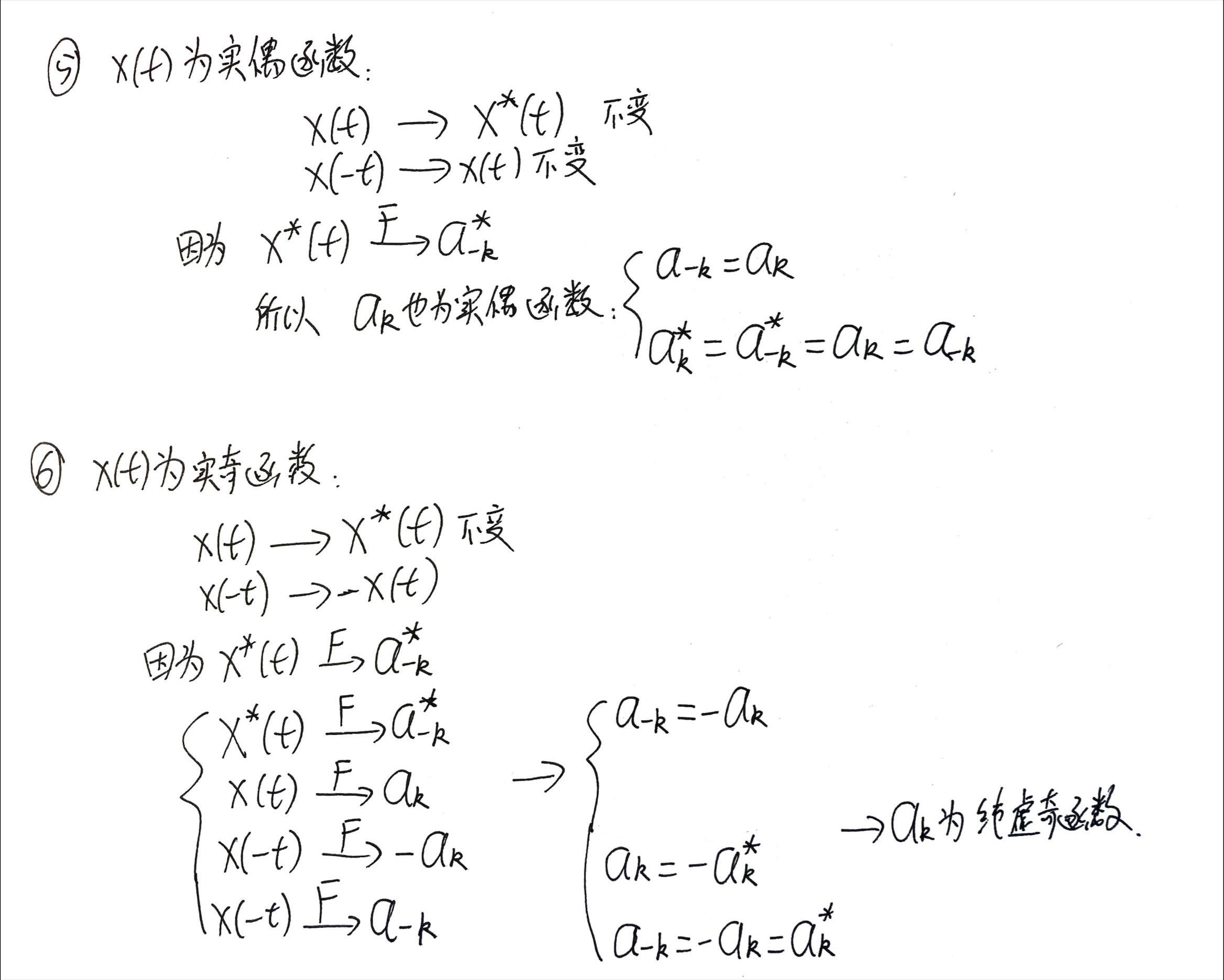
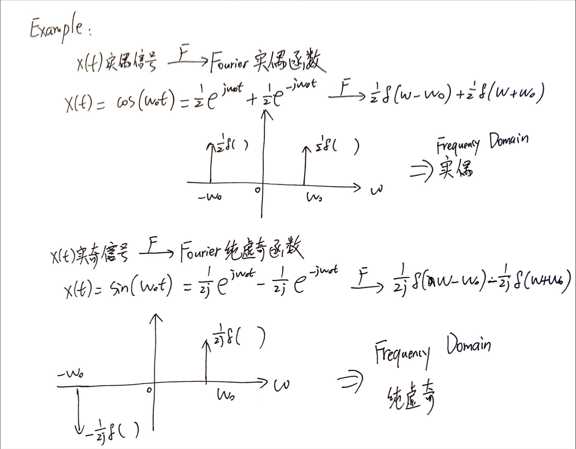
上面只推导了周期连续信号[mathjax]a_k[/mathjax]的情况,非周期连续信号[mathjax]X(j\omega)[/mathjax]的情况应该是基本类似的。
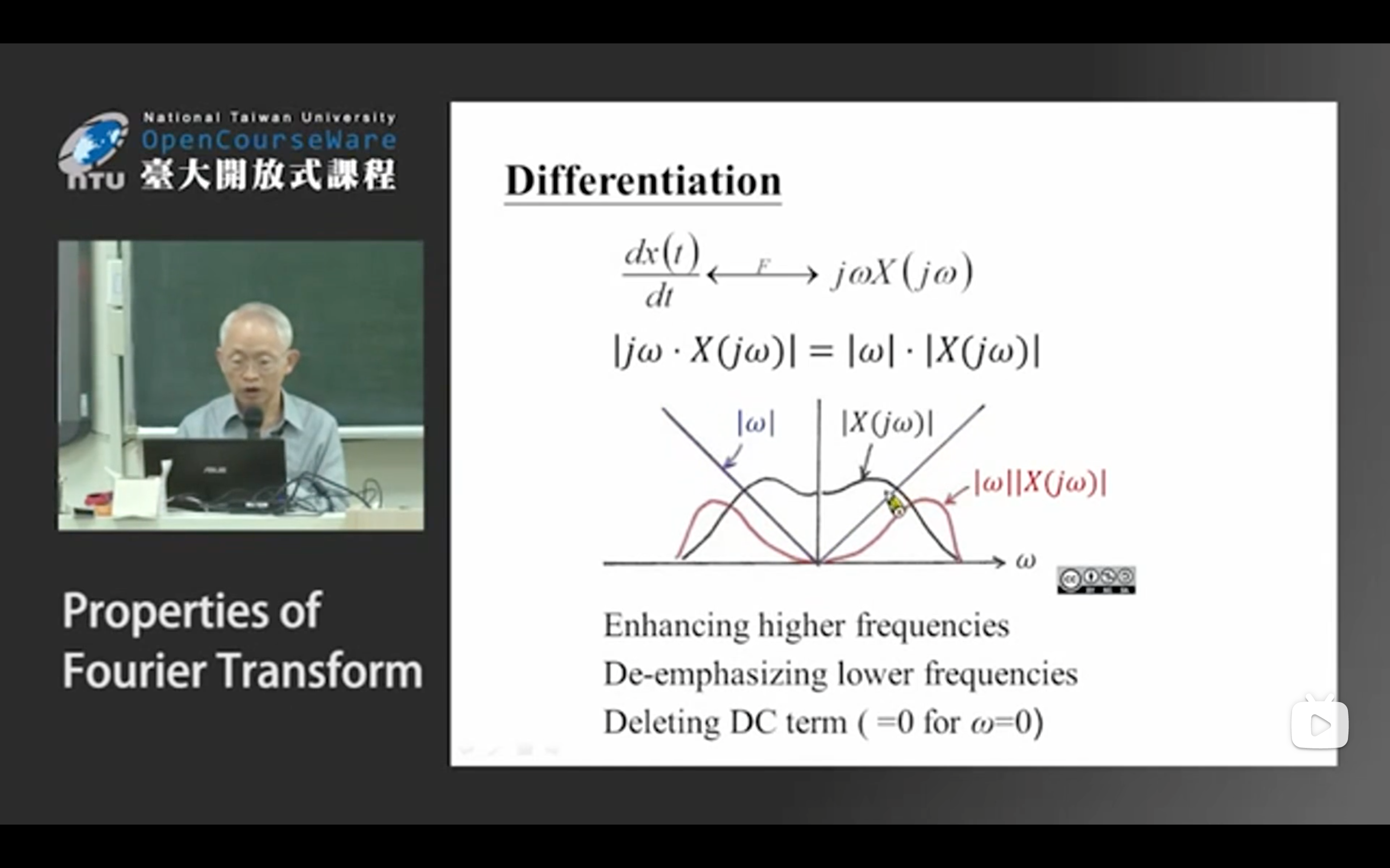
微分和积分
微分和积分
BV1dM4y1M7LK p10 1:00:00左右开始
但在信号与系统的书上暂时没有找到对应的章节
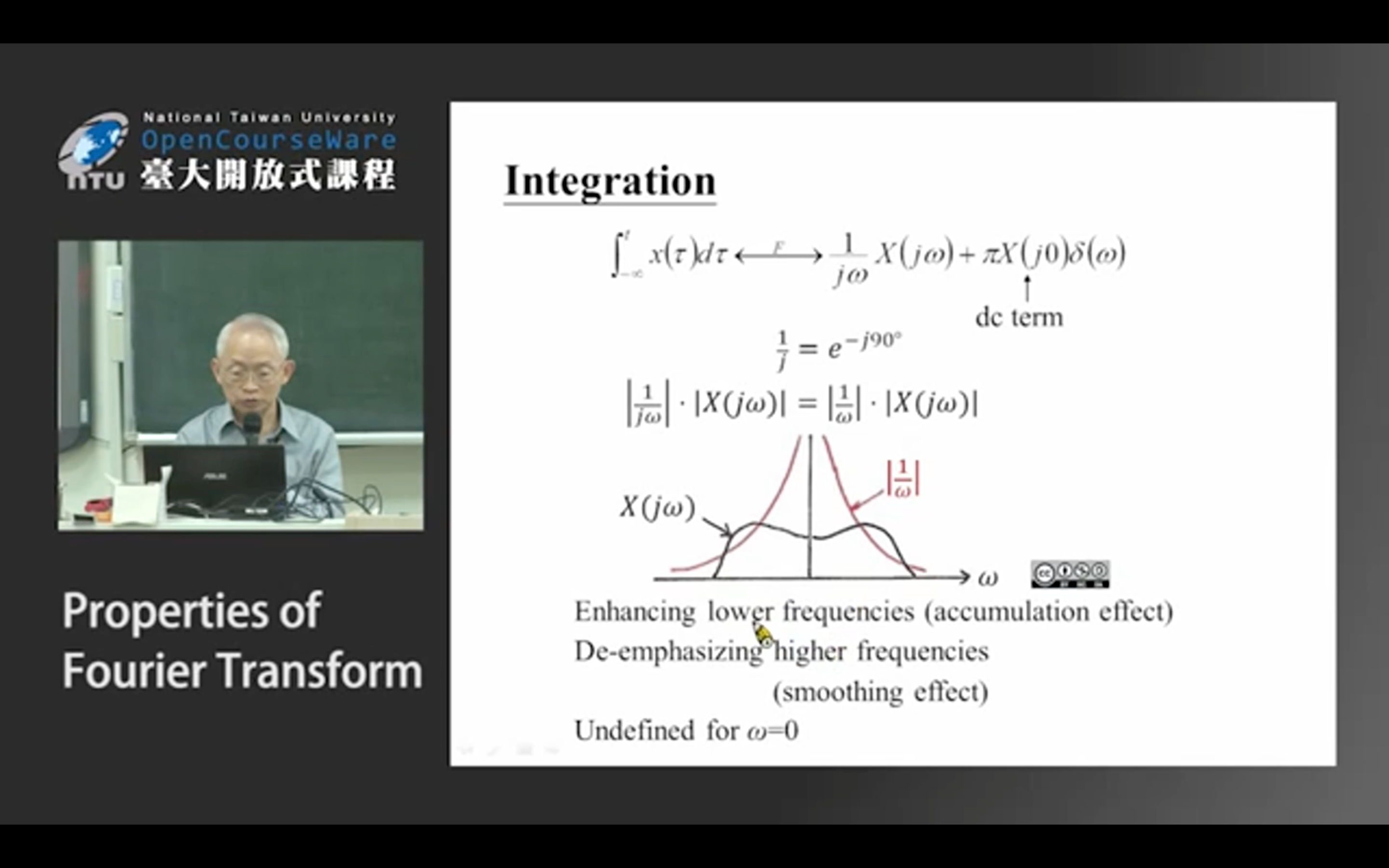
BV1dM4y1M7LK p11 20:00左右开始
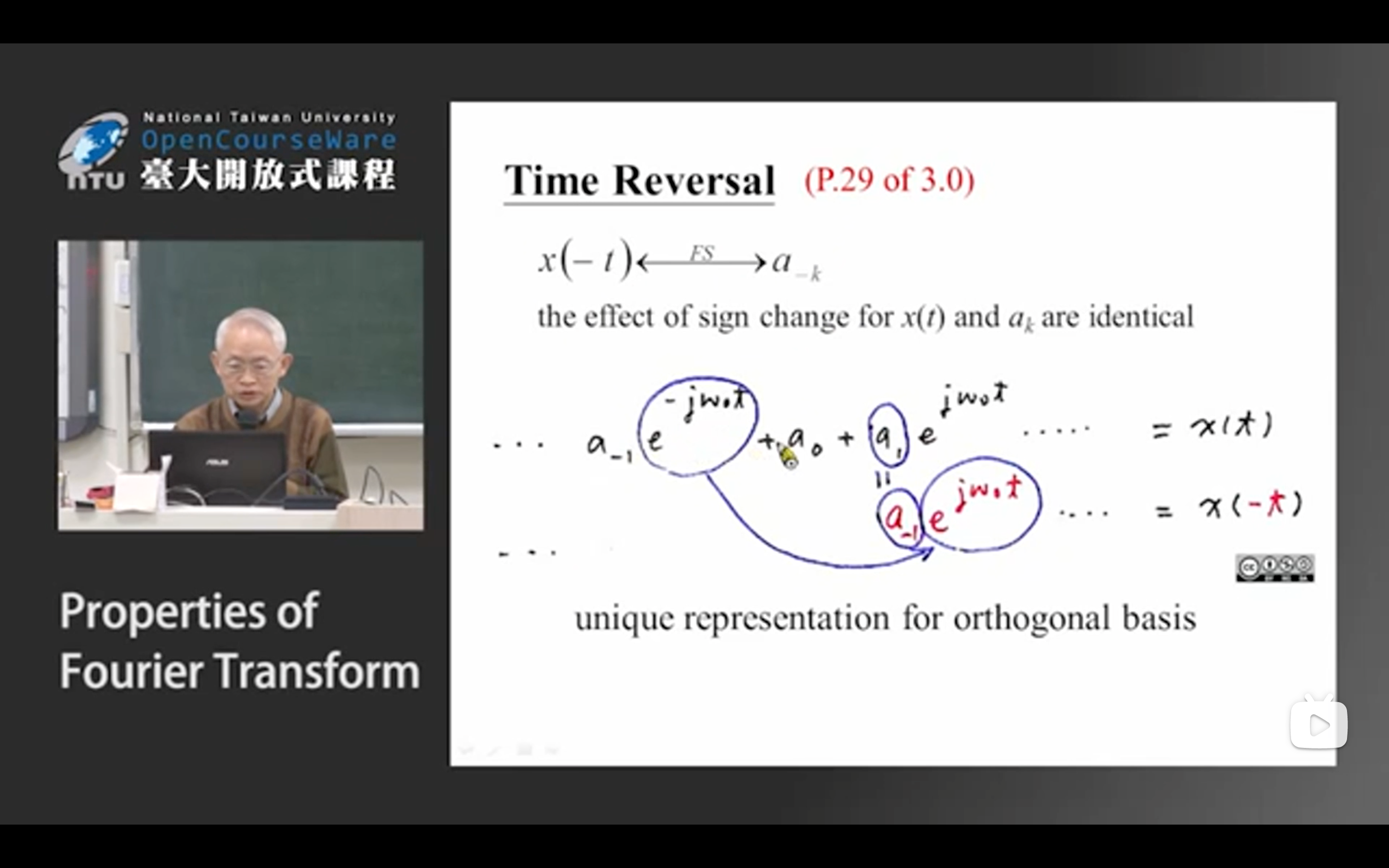
时间反转
时间反转
BV1dM4y1M7LK p11 43:55左右开始
这个比 共轭性质 要简单一些。
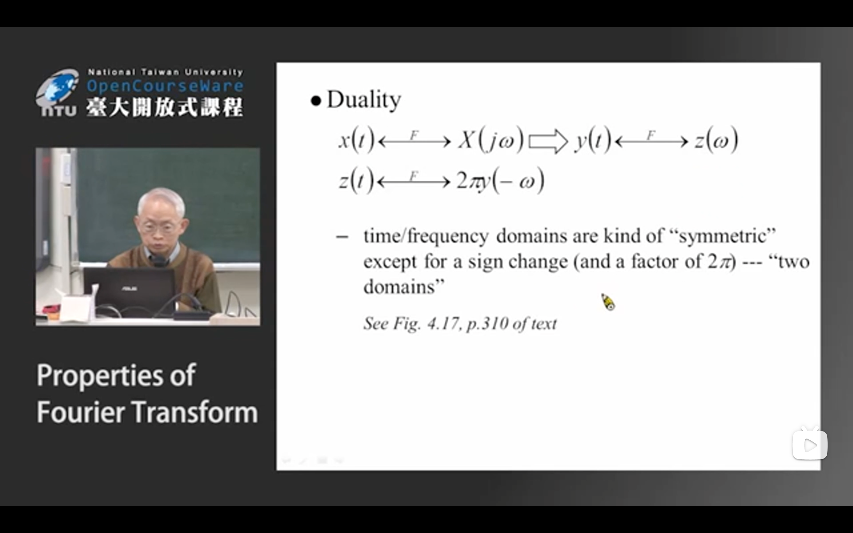
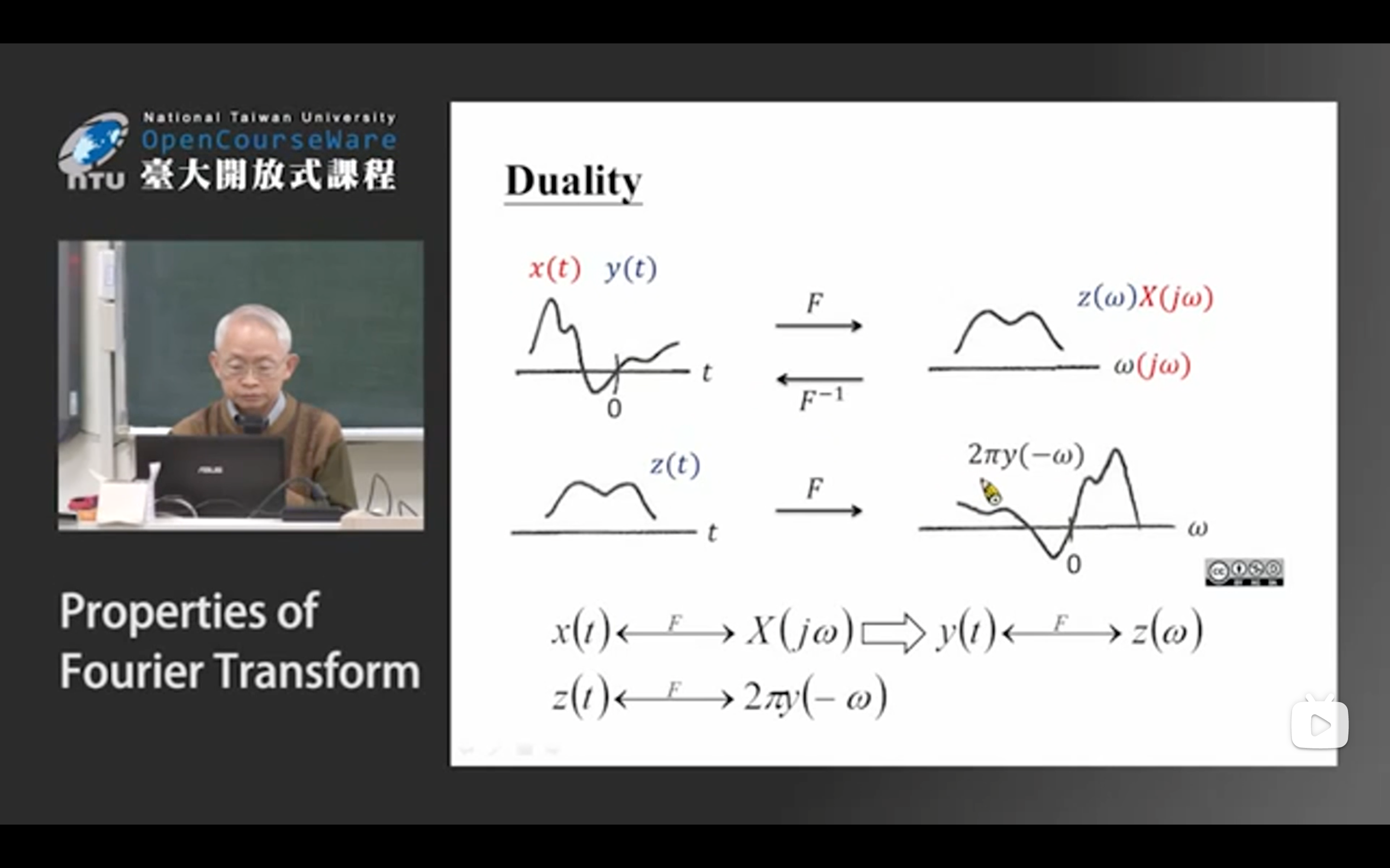
Duality
Duality
BV1dM4y1M7LK p11 55:16左右开始
Modulation property
结合Duality和time shift property,我们可以理解这个:Modulation property(注意要把它和time shift区分开来)
modulation:时域乘以某个复指数信号,导致频域shift
time shift:时域shift,频域也shift(本质上频域是乘以某个复指数,但在频域上体现为shift)
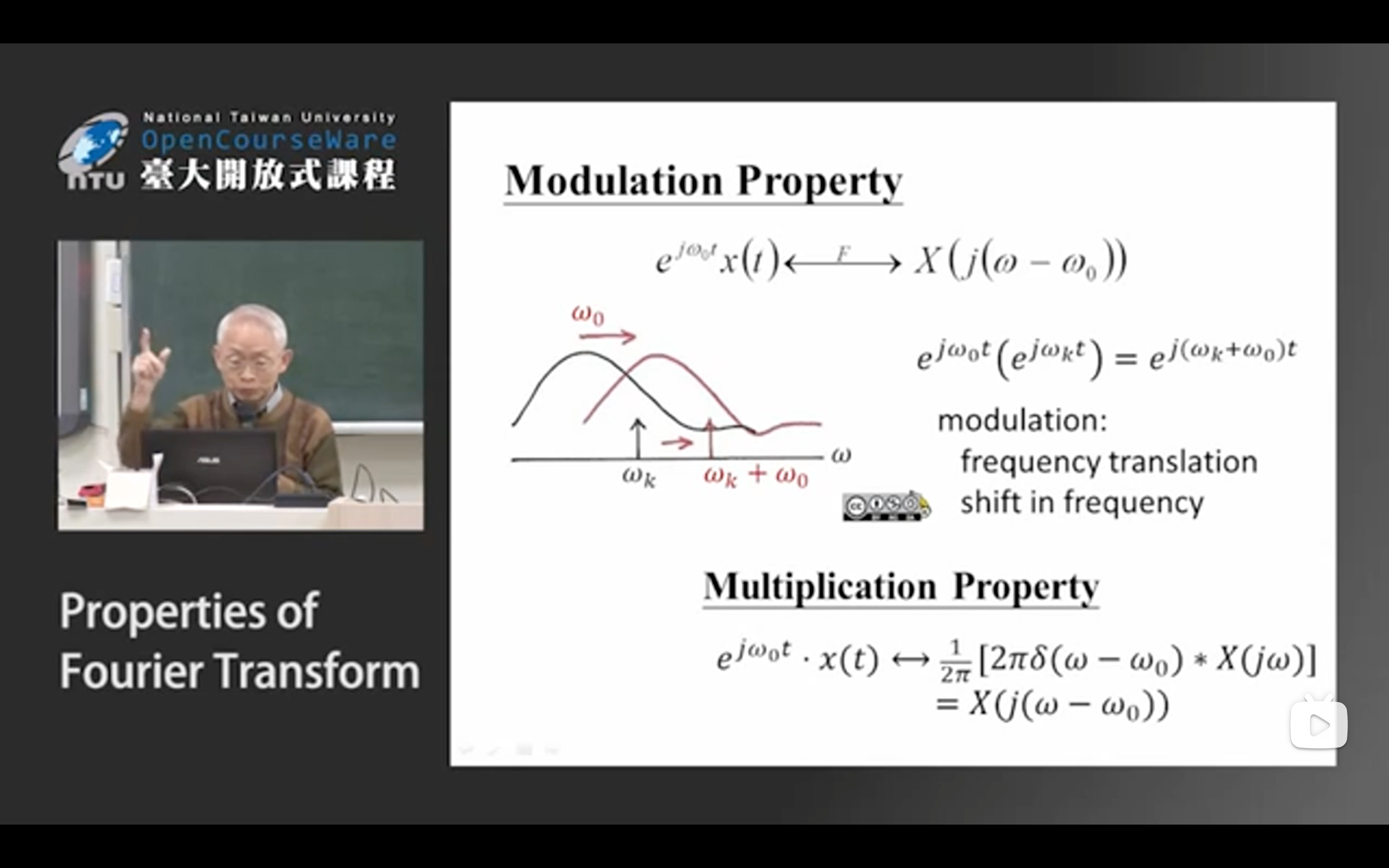
应用场景1:调频通讯
这个在视频里有讲,大概意思就是,两个设备进行无线电通讯,需要把各自的设备都调整到某个相同的基准频率[mathjax]\omega_0[/mathjax]上,这样就需要把传进设备的声音讯号频率进行“frequency shift”,然后再进行传输。
应用场景2:音乐转调
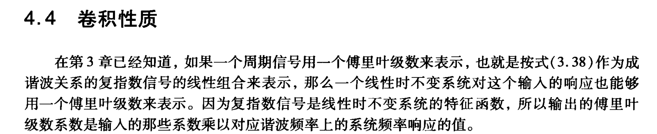
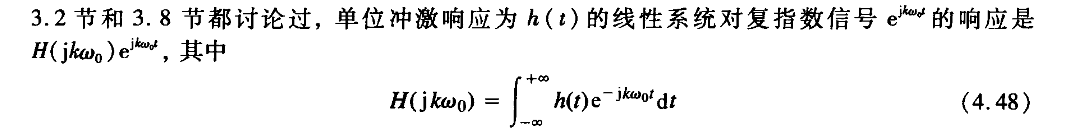
卷积性质
卷积性质
再次尝试一下这个!之前乱学了一通,没有完全学会推导过程。
P199
先讨论一下这个:
需要复习2022-08-28:
以及2022-08-29:
以及🔗 [2022-09-16 - Truxton's blog] https://truxton2blog.com/2022-09-16/
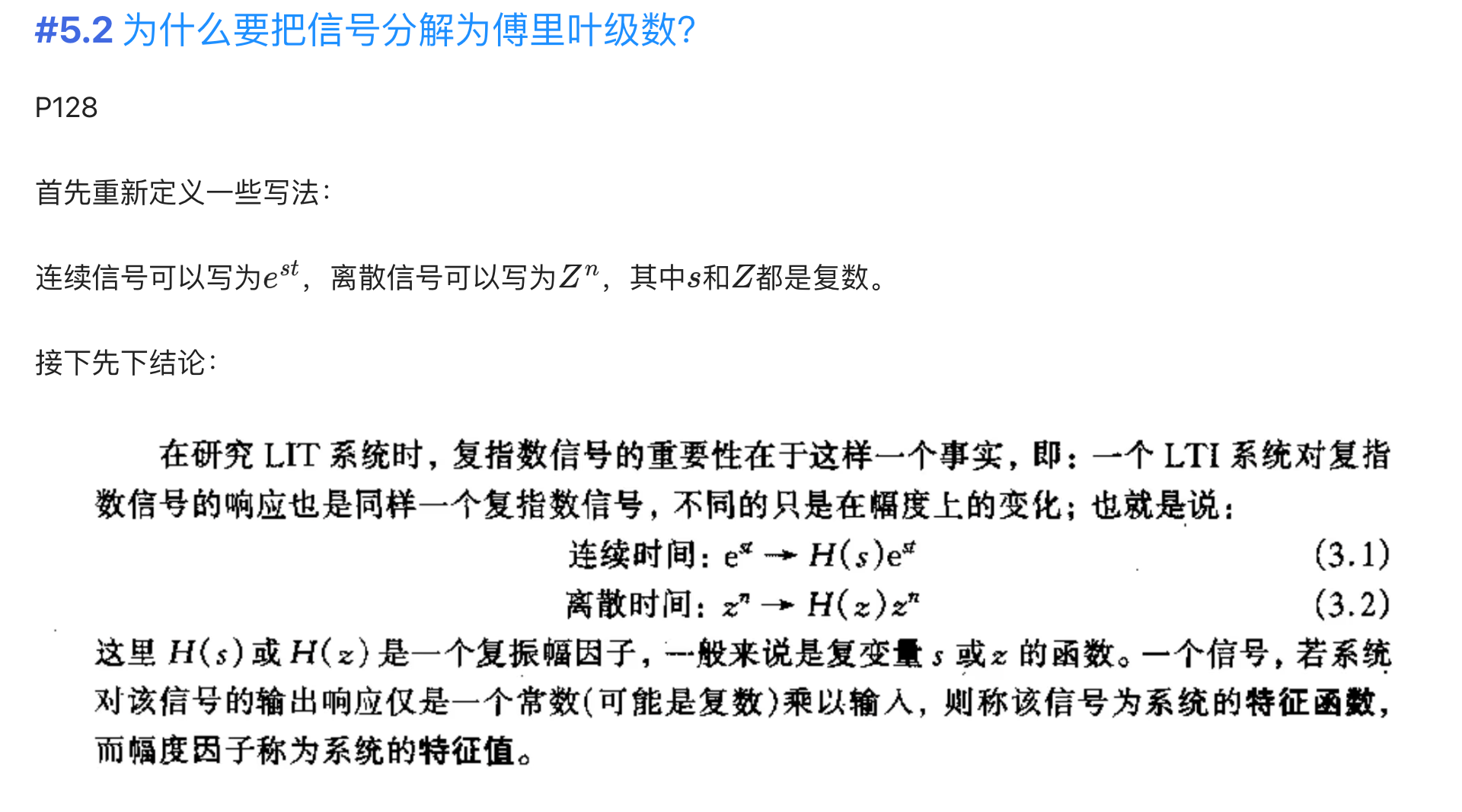
现在暂时抛开书上使用的LTI系统,证明
[mathjax-d]X(j\omega)Y(j\omega)=x(t)*y(t)[/mathjax-d]现在暂时持有结论: 频域相乘,时域卷积
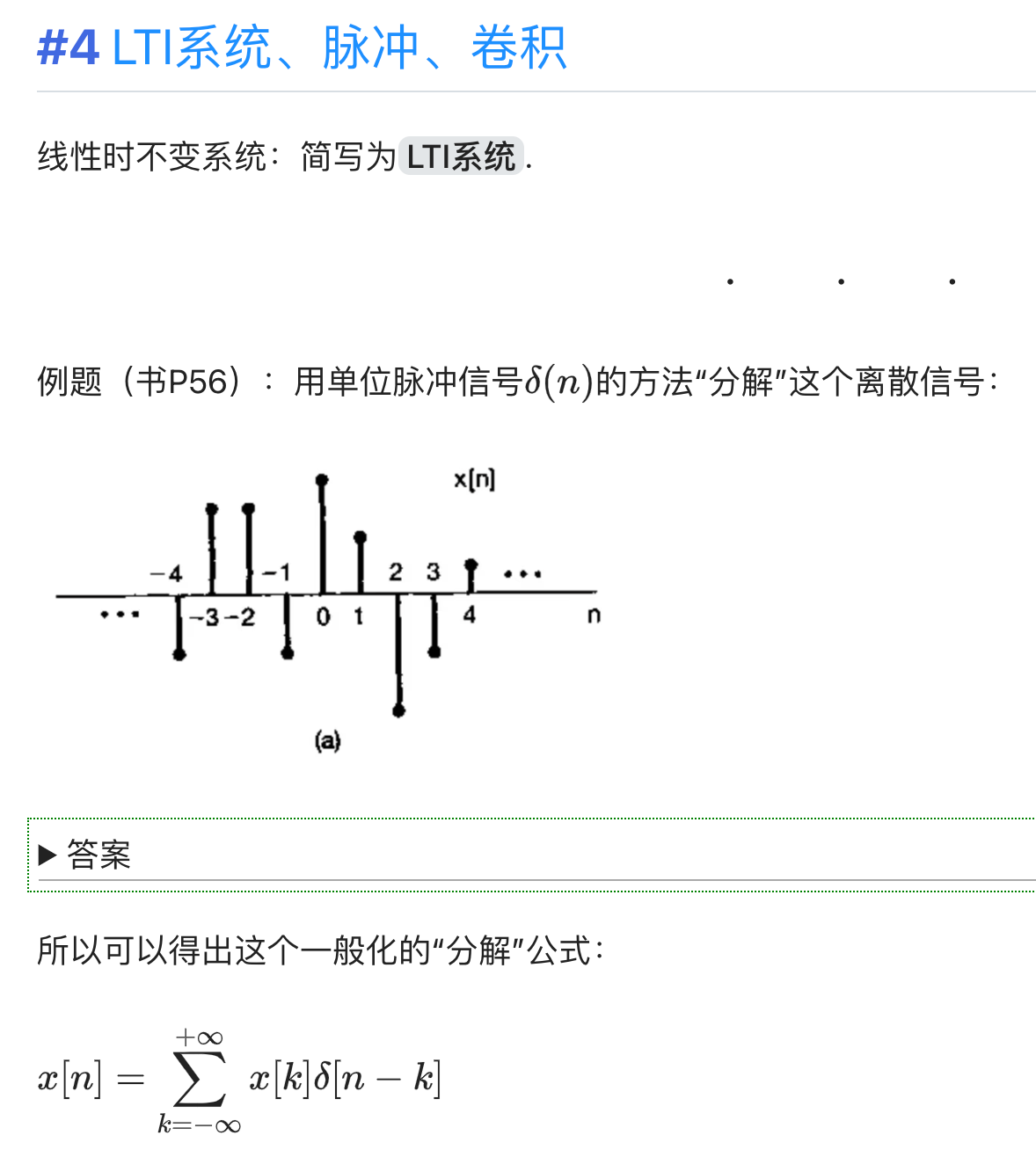
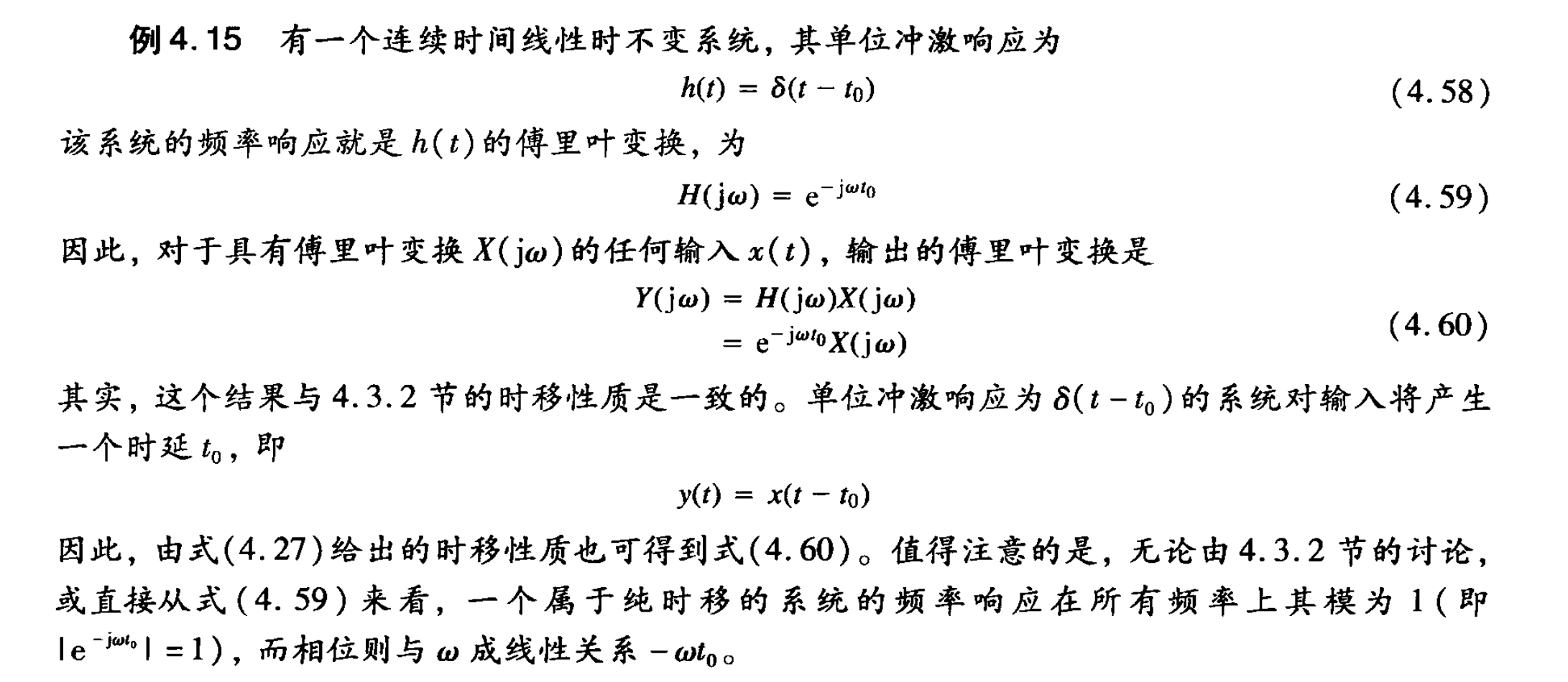
为了防止老年痴呆忘记LTI系统的一些性质,需要回顾这个例题:
非递归离散时间滤波器
一些例题
非递归离散时间滤波器
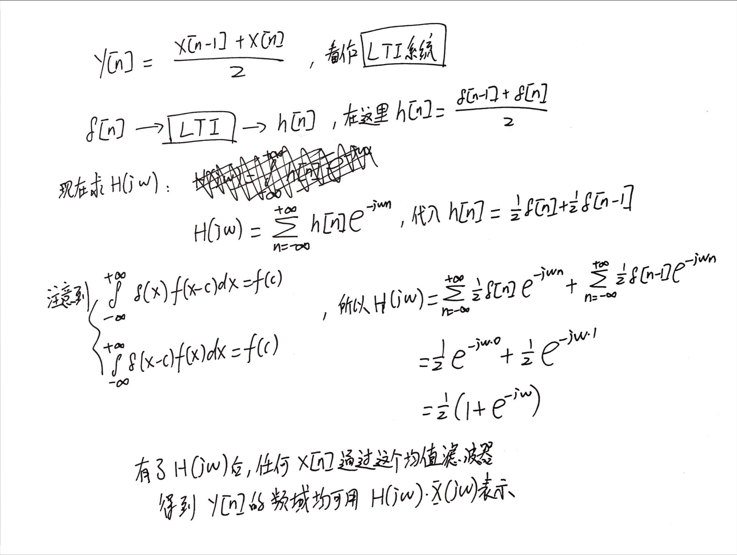
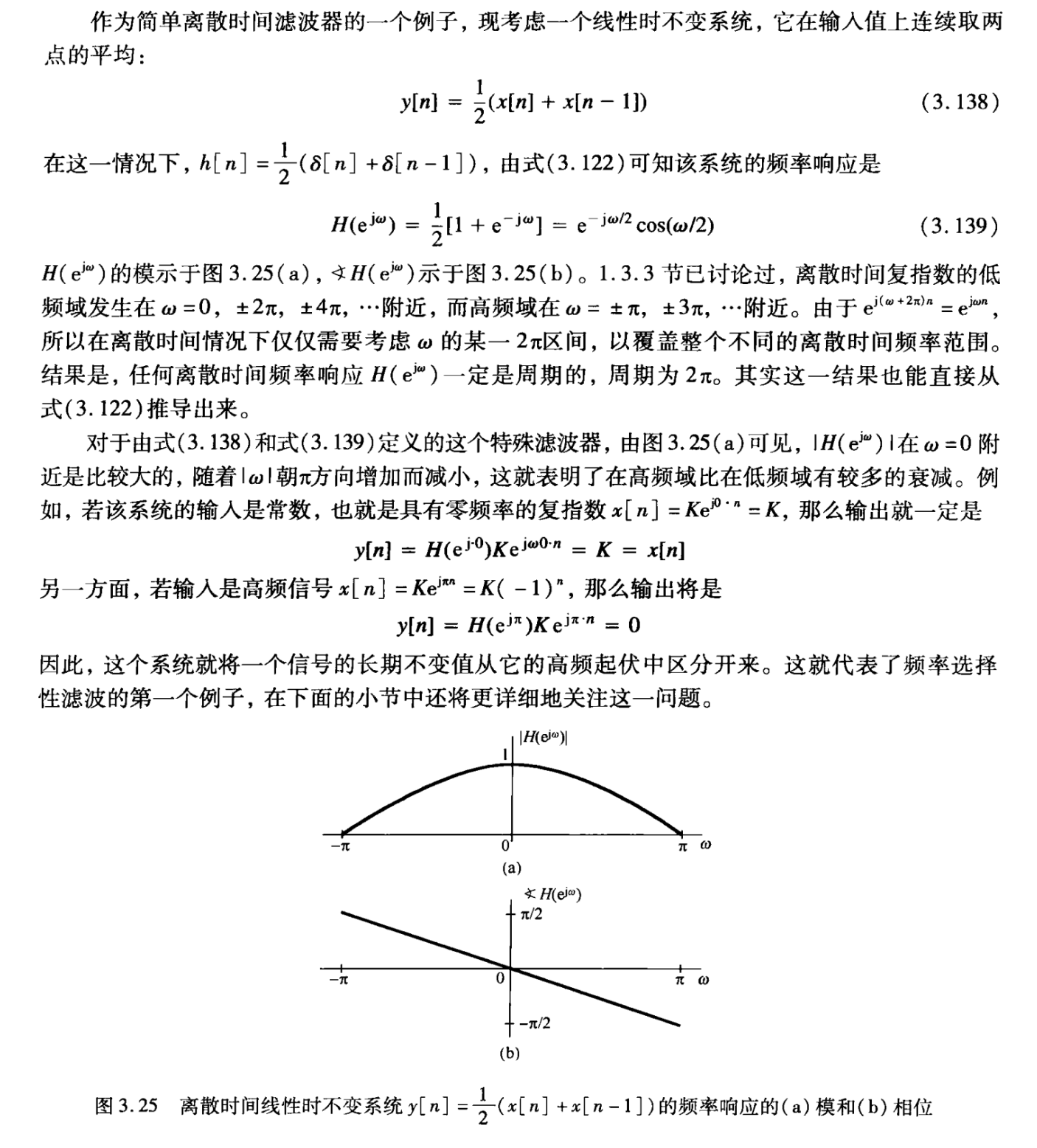
例题1(书P150):有滤波器设计如下:
[mathjax-d]y[n]=\frac{x[n]+x[n-1]}{2}[/mathjax-d]现在要分析这个滤波器对信号产生的效果。
标准答案在书P150:
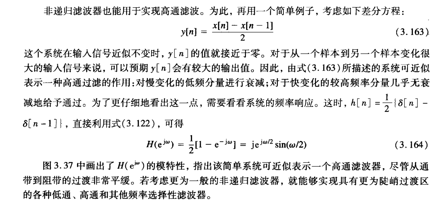
接下来用类似的方法分析这个滤波器(书P158):
[mathjax-d]y[n]=\frac{x[n]-x[n-1]}{2}[/mathjax-d]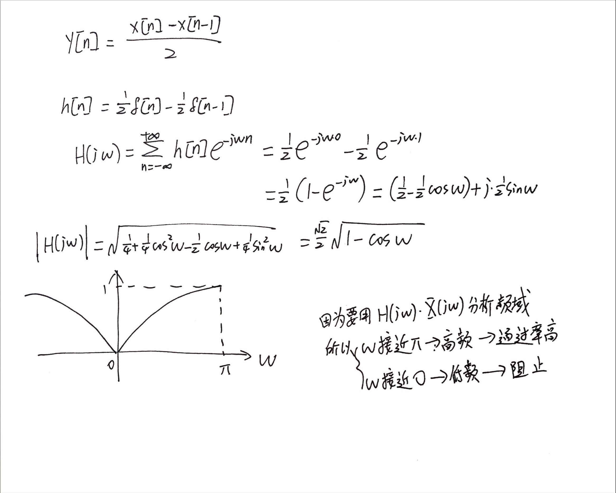
标准答案在书P158~P159:
一些总结
到目前为止学会的 分析滤波器 的方法如下:(连续和离散的情况基本一致,略微修改部分符号即可)
1,想办法得到[mathjax]h(t)[/mathjax]的表达式。上面2道例题可以帮助我们快速学会这个技巧。
2,求[mathjax]h(t)[/mathjax]对应的傅里叶变换表达式:[mathjax]H(j\omega)[/mathjax]
在《信号与系统》中这两个公式分别为3.121和3.122:
[mathjax-d]H(j\omega)=\int_{-\infty}^{+\infty}h(t)e^{-j\omega t}dt[/mathjax-d]以及离散信号版:
[mathjax-d]H(e^{j\omega})=\sum_{n=-\infty}^{+\infty}h[n]e^{-j\omega n}[/mathjax-d]3,得到[mathjax]H(j\omega)[/mathjax]以后,任何通过这个滤波器的信号 的频域 都可以写为[mathjax]H(j\omega)\cdot X(j\omega)[/mathjax] .([mathjax]X(j\omega)[/mathjax]为原本的信号[mathjax]x(t)[/mathjax]对应的傅里叶变换)
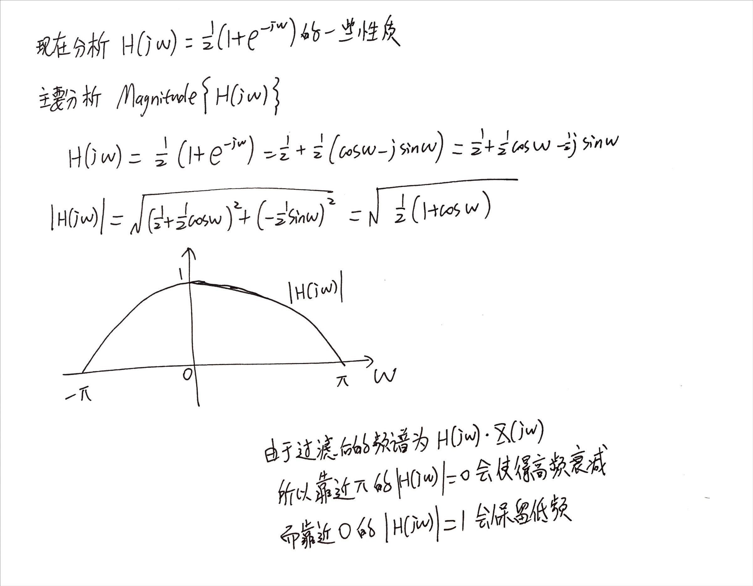
4,绘制出[mathjax]H(j\omega)[/mathjax]对应的模长图[mathjax]\left| H(j\omega) \right|[/mathjax],然后简单进行分析即可。
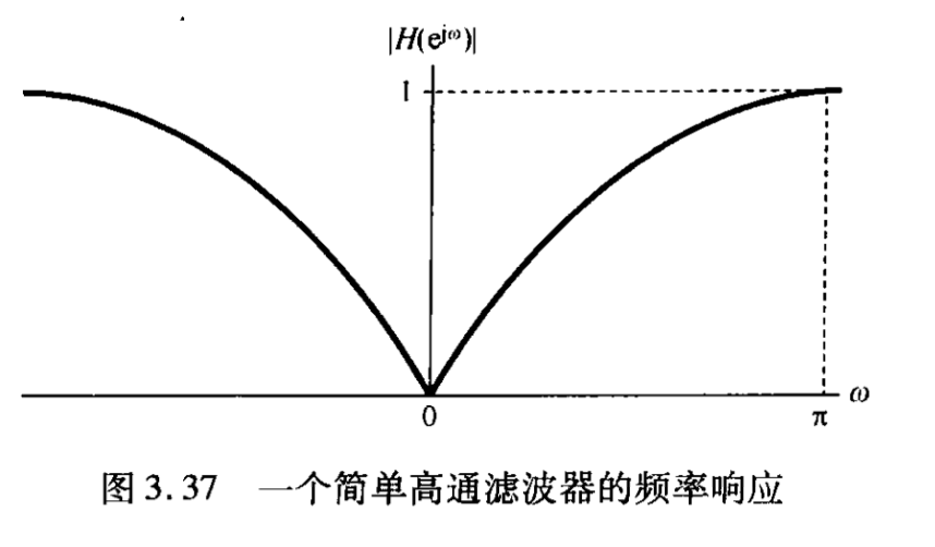
比如,这张[mathjax]\left| H(j\omega) \right|[/mathjax]对应的是高通滤波器,这张[mathjax]\left| H(j\omega) \right|[/mathjax]对应的是低通滤波器。
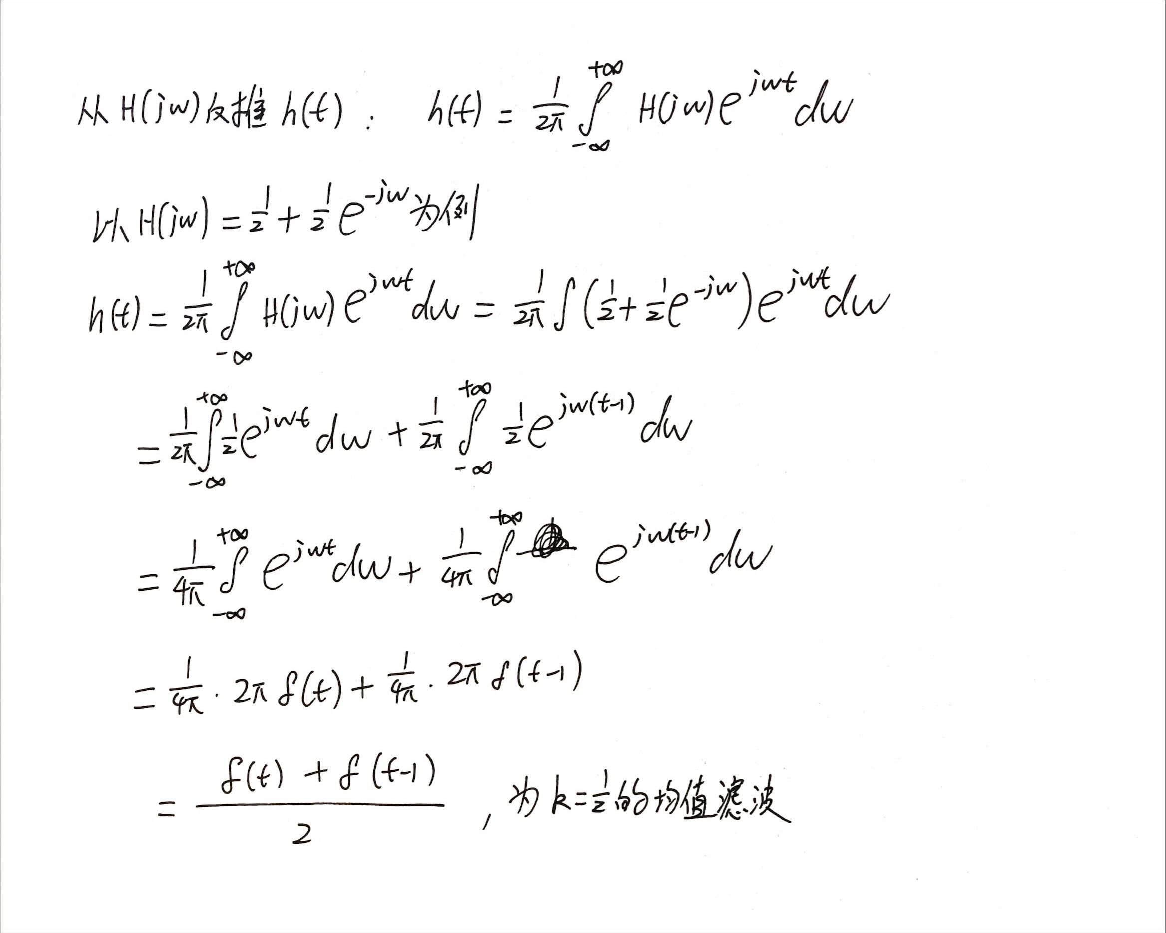
当然,还能从[mathjax]H(j\omega)[/mathjax]反推回[mathjax]h(t)[/mathjax]:
[mathjax-d]h(t)=\frac{1}{2\pi}\int_{-\infty}^{+\infty}H(j\omega)e^{j\omega t}d\omega[/mathjax-d]本质上和 连续非周期信号的傅里叶逆变换 一样。
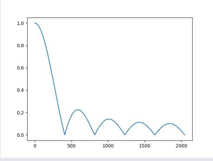
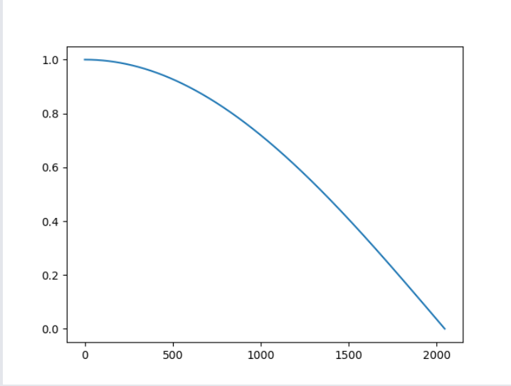
example:
一些代码
import matplotlib.pyplot as plt
import numpy as np

w = np.linspace(0, np.pi, 2048)
h_j_w = 1 / 2 * np.e ** 0 + 1 / 2 * np.e ** (-1j * w * 1)
plt.figure()
plt.plot(np.abs(h_j_w))
plt.show()
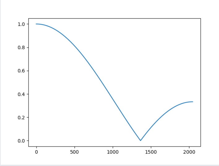
import matplotlib.pyplot as plt
import numpy as np

w = np.linspace(0, np.pi, 2048)
h_j_w = 1 / 3 * np.e ** 0 + 1 / 3 * np.e ** (-1j * w * 1) + 1 / 3 * np.e ** (-1j * w * 2)
plt.figure()
plt.plot(np.abs(h_j_w))
plt.show()
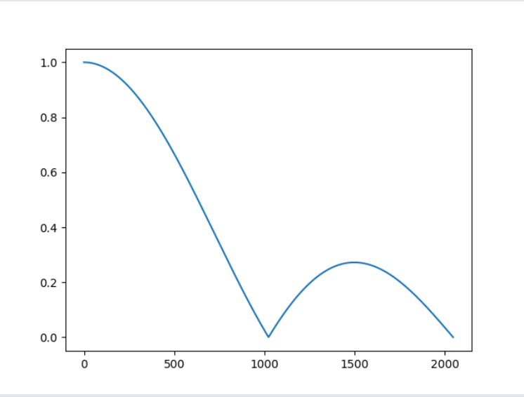
import matplotlib.pyplot as plt
import numpy as np

w = np.linspace(0, np.pi, 2048)
h_j_w = 1 / 4 * np.e ** 0 + 1 / 4 * np.e ** (-1j * w * 1) + 1 / 4 * np.e ** (-1j * w * 2) + 1 / 4 * np.e ** (
            -1j * w * 3)
plt.figure()
plt.plot(np.abs(h_j_w))
plt.show()
import matplotlib.pyplot as plt
import numpy as np

w = np.linspace(0, np.pi, 2048)
h_j_w = 1 / 10 * np.e ** 0 + 1 / 10 * np.e ** (-1j * w * 1) + 1 / 10 * np.e ** (-1j * w * 2) + 1 / 10 * np.e ** (
        -1j * w * 3) + 1 / 10 * np.e ** (-1j * w * 4) + 1 / 10 * np.e ** (-1j * w * 5) + 1 / 10 * np.e ** (
                    -1j * w * 6) + 1 / 10 * np.e ** (-1j * w * 7) + 1 / 10 * np.e ** (-1j * w * 8) + 1 / 10 * np.e ** (
                    -1j * w * 9)
plt.figure()
plt.plot(np.abs(h_j_w))
plt.show()