 WARNING: This article may be obsolete
This post was published in 2021-12-26. Obviously, expired content is less useful to users if it has already pasted its expiration date.
 This article is categorized as "Garbage" . It should NEVER be appeared in your search engine's results.
Table of Contents
主要参考资料
李航《统计学习方法》第二版
周志华《机器学习》
🔗 [Microsoft PowerPoint - mdp.ppt] https://www.cs.cmu.edu/~cga/ai-course/mdp.pdf
预期贴现总和 / expected discounted sum
🔗 [Microsoft PowerPoint - mdp.ppt] https://www.cs.cmu.edu/~cga/ai-course/mdp.pdf
现在看第一页就够了:
这个slide的后续内容留到以后再看。
隐马尔可夫模型 / HMM 的基本概念
✪ 基本概念:李航统计学习方法 p193开始
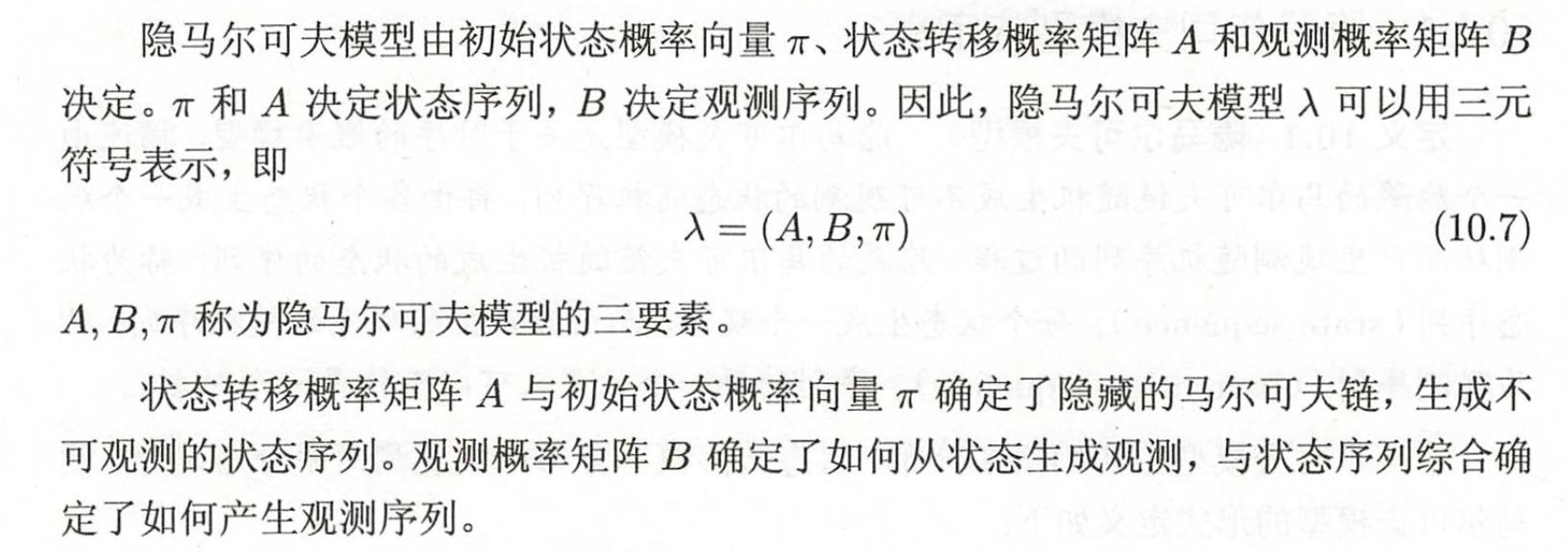
注:“观测概率矩阵[mathjax]B[/mathjax]”的英文名称是emission probabilities,很多中文材料会翻译为“发射概率”。
✪ (如果这个pdf复习不懂,就重新去看书)
✪ 通过这个例子来入门理解HMM的应用:(没有实际题目)
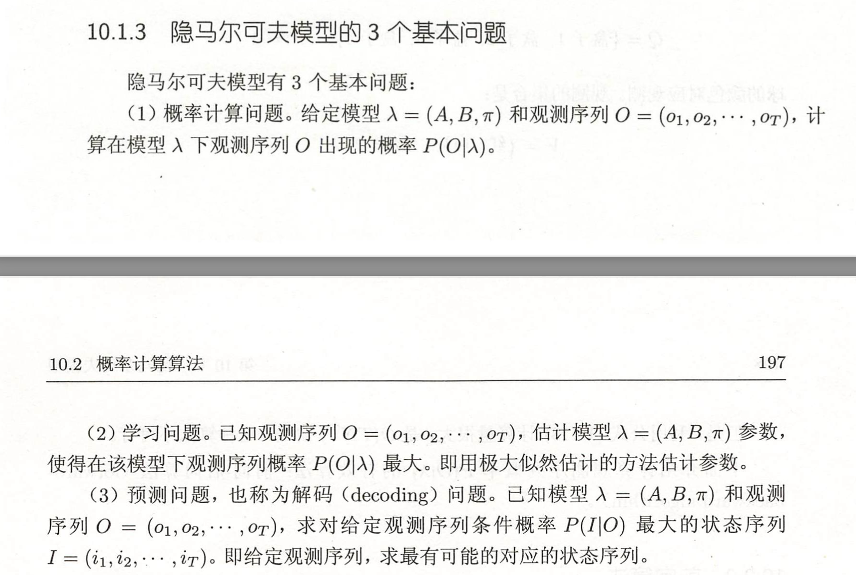
✪ HMM的3个基本问题
马尔可夫决策 / Markov Decision Process 基本概念
马尔可夫决策过程(MDP)是马尔可夫链(MC/MP)的推广。
MDP的目标(简单的说):找到一个好策略,使得收益最大化。
✪ wikipedia的例子(奖励绑定动作)
注意:接下来的例子被限定为奖励绑定动作,区别于后续的奖励绑定状态
🔗 [马尔可夫决策过程 - 维基百科,自由的百科全书] https://zh.wikipedia.org/zh-hans/馬可夫決策過程
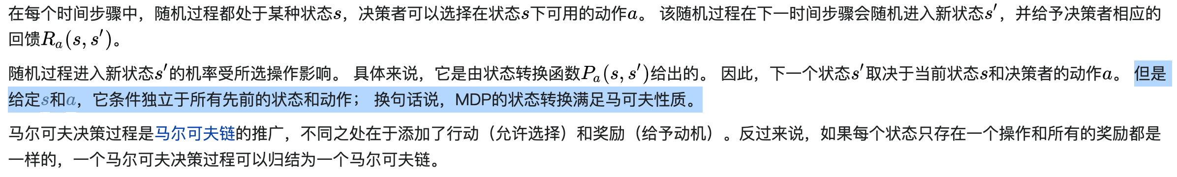
一个简单的MDP示例,包含三个状态(绿色圆圈)和两个动作(橙色圆圈),以及两个奖励(橙色箭头)。

在MDP开始之前,有[mathjax]P_{a}\left(s, s^{\prime}\right)=\operatorname{Pr}\left(s_{t+1}=s^{\prime} \mid s_{t}=s, a_{t}=a\right)[/mathjax],代表是[mathjax]t[/mathjax]时刻[mathjax]s[/mathjax]状态下的动作[mathjax]a[/mathjax]导致[mathjax]t+1[/mathjax]时刻进入状态[mathjax]s'[/mathjax]的概率。
在MDP开始以后,原先的[mathjax]P_{a}\left(s, s^{\prime}\right)=\operatorname{Pr}\left(s_{t+1}=s^{\prime} \mid s_{t}=s, a_{t}=a\right)[/mathjax]就会变成[mathjax]\operatorname{Pr}\left(s_{t+1}=s^{\prime} \mid s_{t}=s\right)[/mathjax]. 比如:从[mathjax]S_2[/mathjax]出发到[mathjax]S_0[/mathjax],原本可以经过动作[mathjax]a_1[/mathjax]或者[mathjax]a_0[/mathjax],但现在只有1种固定的途径,因为[mathjax]\pi(s)[/mathjax]决定了状态[mathjax]s[/mathjax]的动作。所以MDP的目标就是找到一个策略[mathjax]\pi[/mathjax],在状态为[mathjax]s[/mathjax]的时候为这个状态指定一个动作[mathjax]\pi(s)[/mathjax] . 这个策略[mathjax]\pi[/mathjax]的目的就是让随机奖励的累积函数最大化,通常是在潜在的无限范围内的预期贴现总和:[mathjax]E\left[\sum\limits_{t=0}^{\infty} \gamma^{t} R_{a_{t}}\left(s_{t}, s_{t+1}\right)\right][/mathjax] . 解释:从状态[mathjax]s_t[/mathjax]到状态[mathjax]s_{t+1}[/mathjax],策略[mathjax]\pi(s)[/mathjax]规定了执行动作[mathjax]a[/mathjax],所以这个转移步骤对应了奖励[mathjax]R_{a_{t}}(s_t,s_{t+1})[/mathjax] . 如果[mathjax]s_t[/mathjax]是已经确定的,那么有且只有一种可能的奖励值[mathjax]R_{a_{t}}(s_t,s_{t+1})[/mathjax]. 再考虑折现因子[mathjax]\gamma[/mathjax]的影响,把每一步的奖励进行累加,就可以得到随机奖励的累积函数。 如果[mathjax]\gamma[/mathjax]比较低,就会促使决策者倾向于尽早采取行动,而不是无限期地推迟行动。(见本文开头的预期贴现总和)
马尔可夫决策 计算方法
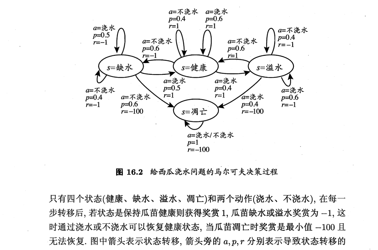
✪ 奖励绑定状态
在上面的wikipedia例子中,每一个动作对应了一个奖励;现在(包括接下来的内容)改为讨论“每一个状态对应了一个奖励”,比如:
✪ 递推公式
首先是之前出现的:[mathjax]E\left[\sum\limits_{t=0}^{\infty} \gamma^{t} R_{a_{t}}\left(s_{t}, s_{t+1}\right)\right][/mathjax],将它进行修改:
从状态[mathjax]S_i[/mathjax]开始计算,首先它拥有一个奖励(因为“奖励绑定状态”),然后它需要转移到下一个状态[mathjax]S_j[/mathjax]上:这个[mathjax]S_j[/mathjax]有可能是[mathjax]\left\{S_{1},\ S_{2}, \cdots ,\ S_{N}\right\}[/mathjax]中的任意一个(包括自己),每一个可能的[mathjax]S_j[/mathjax]都对应一个转移概率(转移矩阵中的一行),但是在计算的时候需要乘以折现因子:
[mathjax-d]\displaylines{\mathrm{J}^{*}\left(\mathrm{~S}_{j}\right)=r_{i}+\gamma \mathbf{x} \cr \mathbf{x}:\text{ Expected future rewards starting from your next state}}[/mathjax-d]也就是:
[mathjax-d]\mathrm{J}^*(\mathrm{S}_i)=r_i+\gamma (P_{i1}\mathrm{J}^*(\mathrm{S}_1^{\prime})+P_{i2}\mathrm{J}^*(\mathrm{S}_2^{\prime})+\ \cdots \ P_{iN}\mathrm{J}^*(\mathrm{S}_N^{\prime}))[/mathjax-d](在这里[mathjax]\mathrm{S}^{\prime}[/mathjax]表示状态[mathjax]\mathrm{S}[/mathjax]的下一次转移状态)
✪ 暂停一下
我在继续思考MDP的时候曾经陷入过一个巨大的误区:我似乎完全忽略了【决策】这一重要因素(因为一开始画图的时候没有画仔细,把决策漏画了,所以MDP就变成了一个普通的马尔可夫),所以我一时无法理解下面这个公式中,[mathjax]P^k_{ij}[/mathjax]的[mathjax]k[/mathjax]到底是什么:
[mathjax-d]\arg \max _{k}\left[r_{i}+\gamma \sum_{j} \mathrm{P}_{i j}^{k} \mathrm{~J}^{*}\left(\mathrm{~S}_{j}\right)\right][/mathjax-d]事实上[mathjax]P^k_{ij}[/mathjax]代表的是“多个马尔可夫状态转移表中的一个”,也就是一个决策:从状态[mathjax]\mathrm{S}[/mathjax]出发,可能会有不止1个决策,每个决策都分别对应了转移概率矩阵[mathjax]\boldsymbol{P}[/mathjax]中的一行。
✪ 参考资料
来源:🔗 [Microsoft PowerPoint - mdp.ppt] https://www.cs.cmu.edu/~cga/ai-course/mdp.pdf
但要注意,Slide 16似乎有一个地方写错了
OCR辅助查找工具
Prediction and Search in Probabilistic Worlds Markov Systems, Markov Discounted RewardsDecision Processes, and An assistant professor gets paid, say, 20K per year.Dynamic Programming How much. in total. will the 4.P earn in their life? 20+20+ 20+20+20+.= InfinityRone to cther toacters ond uersof ryou fcurd hls gcurce moteribs wetulh Andrew W. MooreP S SR H: Associate Professor to nt Yeuro o a sgrifcant porticn st thee slbes in S R.REE School of Computer Sciencesurce repostory ot Andkeers Putorols: Carnegie Mellon UniversityCenee cekg eedauy www.cs.cmu.edu/~awmFO0OwS avm@cs.cmu.edu 412-268-7599 What’s wrong with this argument?Copyrignt & 2002, Andrew W. Moore Aorll 21gt. 2002 Copyrign ® 2002. Andrear W. Moore Markey Sygtems: slide 2Discounted Rewards Discount Factors‘A reward (payment) in the future is not worth quite aS much as a reward now.” People in economics and probabilistic decision-• Because of chance of obliteration making do this all the time.Because of inflation The “Discounted sum of future rewards” usingExample: discount factor y’ isBeing promised $10,000 next year is worth only 90% as (reward now) +much as receiving $10,000 right now. Assuming payment n years in future is worth only Y(reward in 1 time step) +(0.9)/ of payment now, what is the AP’s Future y (reward in 2 time steps) +Discounted Sum of Rewards? y3 in (reward in 3 time steps) +Copynghk & Ardrew W. Mocre (infinite sum)Markov Sysioms:s Copyihto Andrewr W. Woore Syatema: sldo 4The Academic Life Computing the Future Rewards of an0.2 AcademicAssistant ASSOC Prof 20 Prof Tenured 60 Prof 4000.2、 On the D. 0.3Street Define: D.7 10 Dscou0.3 AS9Um.209. Factor. JA = Expected discounted future rewards starting in state A Je= Expected discounted future rewards starting n state B JT= Js TJo= 4 SHow do we compute Ja, Je. JT. Js. Jo? DCopmiel s 2002. Andkrew Vi. Moore Markov Systems: Side 5 Copyignt® 2002, Andrear W. Moore Markoy Syatemrs: slide 6—隐马尔可夫模型由初始状态概率向量丌、状态转移概率矩阵A和观测概率矩阵B决定。元和A决定状态序列,B决定观测序列。因此,隐马尔可夫模型入可以用三元符号表示,即入=(A, B,T) (10.7) A,B,元称为隐马尔可夫模型的三要素。状态转移概率矩阵A与初始状态概率向量『确定了隐藏的马尔可夫链,生成不可观测的状态序列。观测概率矩阵B确定了如何从状态生成观测,与状态序列综合确定了如何产生观测序列。10.1隐马尔可夫模型的基本概念195隐马尔可夫模型可以用于标注,这时状态对应着标记。标注问题是给定观测的序列预测其对应的标记序列。可以假设标注问题的数据是由隐马尔可夫模型生成的。这样我们可以利用隐马尔可夫模型的学习与预测算法进行标注。下面看一个隐马尔可夫模型的例子。例10.1(盒子和球模型)假设有4个盒子,每个盒子里都装有红、白两种颜色的球,盒子里的红、白球数由表10.1列出。表10.1各盒子的红、白球数盒子1 2 3红球数5 6白球数5 4 2按照下面的方法抽球,产生一个球的颜色的观测序列: •开始,从4个盒子里以等概率随机选取1个盒子,从这个盒子里随机抽出1个球,记录其颜色后,放回: 。然后,从当前盒子随机转移到下一个盒子,规则是:如果当前盒子是盒子1,那么下一盒子一定是盒子2:如果当前是盒子2或3,那么分别以概率0.4和0.6转移到左边或右边的盒子:如果当前是盒子4,那么各以0.5的概率停留在盒子4或转移到盒子3;确定转移的盒子后,再从这个盒子里随机抽出1个球,记录其颜色,放回:如此下去,重复进行5次,得到一个球的颜色的观测序列:◎=(红,红,白,白,红)在这个过程中,观察者只能观测到球的颜色的序列,观测不到球是从哪个盒子取出的,即观测不到盒子的序列。在这个例子中有两个随机序列,一个是盒子的序列(状态序列),一个是球的颜色的观测序列(观测序列)。前者是隐藏的,只有后者是可观测的。这是一个隐马尔可夫模型的例子。根据所给条件,可以明确状态集合、观测集合、序列长度以及模型的三要素。盒子对应状态,状态的集合是:Q={盒子1,盒子2,盒子3,盒子4,N=4球的颜色对应观测。观测的集合是:V={红,自),M=210.1.3隐马尔可夫模型的3个基本问题隐马尔可夫模型有3个基本问题: (1)概率计算问题。给定模型入=(A,B,)和观测序列◎=(o1,02,•,or),计算在模型入下观测序列◎出现的概率P(OIA)。10.2概率计算算法197(2)学习问题。己知观测序列◎=(o1,02,⋯,or),估计模型入=(A,B,不)参数,使得在该模型下观测序列概率P(OIA)最大。即用极大似然估计的方法估计参数。 (3)预测问题,也称为解码(decoding)问题。已知模型入=(A,B,元)和观测序列◎=(ol,02,⋯,0T),求对给定观测序列条件概率P(IIO)最大的状态序列1=(a1,a2,,)。即给定观测序列,求最有可能的对应的状态序列。a=不浇水a=浇水D=0.4 p=0.6 a=浇水7=1 r=1 p-0.5 G=不浇水)=-1 =不浇水P=0.4 =0.6 a=不浇水p=0.6 7=-1S=缺水s=健康s=溢水a=浇水a=浇水a=不浇水p=0.5 p=0.4 p=0.4 a=不浇水=浇水a=浇水r=-1 p=0.6 )=-100 S=凋亡p=0.4 p=0.6 r--1 r=-100a=浇水/不浇水P=1 )=-100图16.2给西瓜浇水问题的马尔可夫决策过程只有四个状态(健康、缺水、溢水、凋亡)和两个动作(浇水、不浇水),在每一步转移后,若状态是保持瓜苗健康则获得奖赏1,瓜苗缺水或溢水奖赏为一1,这时通过浇水或不浇水可以恢复健康状态,当瓜苗调亡时奖赏是最小值—100且无法恢复.图中箭头表示状态转移,箭头旁的a,p,r分别表示导致状态转移的注意这里的了”(S)和Sick 2o份T(9)定不同 A Markov System with Rewards… Solving a Markov System Has: set of states (S,S, •Sa Write J(S) = expected discounted sum of future rewards Has a transition probability matrix starting in state S, Pr P12 PIN J(S) =,+ y X (Expected fuure rewards starting from next state) Pa Pe= Prob(Next = S,I This = S) =「+YPrJ(S1)+P2J(S2)+ •PNJ(Sw)) Pr Paw Using vector notation write Each state has a reward. (ra f2 - IN} J(S) 1 11 P12 P1N There’s a discount factor y. 0<¥≤1 J(s,} On Each Time Step J= 2 D 21 . O. Assume your state is S, J(SN) R= P= N PN1 PN2° PNN 1. You get given reward r, 2. You randomly move 1 another state P(NextState = S,I This S)=P, Question: can you invent a closed form expression for J in terms of R P and y? 3. All future rewards are discounted byY Copyigh $ 2002 Andrew Vi. Moore Markov Systems: Side 7 Copyrignt o 2002. Andrew W. Mooce Markow Syatem: slide 8 Solving a Markoy System with Matrix Solving a Markov System with Matrix Inversion Inversion Upside: You get an exact answer Upside: You get an exact answer Downside: Downside: If you have 100,000 states you’re solving a 100,000 by 100,000 system of equations. Copynighk & Ardrew W. Mocre Markav Systams: Side Copwnight o: AndtGwW woore y Syatems: Slido 10 Value Iteration: another way to solve Value Iteration: another way to solve a Markov System a Markov System Define Define J’(S) = Expected discounted sum of rewards over the next 1 time step. J (S) = Expected discounted sum of rewards over the next 1 time step. J2(S) = Expected discounted sum rewards during next steps J2(S) = Expected discounted sum rewards during next 2 steps J’(S) = Expected discounted sum rewards during next steps J(S) = Expected discounted sum rewards during next 3 steps J(S) = Expected discounted sum rewards during next k steps JK(S) = Expected discotnted sim.rewards during next k steps N= Number of states J’(S)= (what?) JS)=r; (what?) J(S)= (what?) J(S) = 1+Zp,J(s) (what?) Jt(S)= (what?)兴J(S)=4+≥P,J(s) (what?) Coprigl e 2002., Prdrew w. Mocre Marxow Syssems: side 1 i=1 Copyrignt e 2002, Andrerw W. Moore Markoy Syatemsr slide 12 2 Value Iteration for solving Markov Let’s do Value Iteration Systems 1/2 NINC /2 Y=0.5 Compute J’(S) for eachj HAIL : Compute J2(S) for eachj -8 k J(SUN) JK(WIND) J(HAIL) Compute J(S) for eachj As k一∞ JK(S)一J(S). Why? 1 When to stop? When 2 Max J1(S) - JK(S) S 3 4 This is faster than matrix inversion (N& style) 5 the transition matrix is sparse : Slde 13 Copyignto 2002. Andrew w. Voor Markoy Systems: slide 14 Copyighx s 2002, Anckew W. Moore Marko s A Markov Decision Process Markov Decision Processes An MDP has… You run a A set of states (s . SNl startup Poor Poori company. Unknown Famous A set of actions fa,⋯ ast should be Sq, a Qn? A set of rewards fr I (one for each state) In every A transition probability function you must choose 1/2 P Prob(Next = jThis =iand use action K) between Saving each step: money or 1/2 Rich & D. Call current state S, Advertising. Rich& 1. Receive reward r Unknown Famous F10 Choose action e fa, • aw 3. you choose action a youll state S, with probability PA 4. All future rewards are discounted byY Syase Copyrigh & 2002, Ardrew W. Mocre Marsov Sysvems: si Copyright o 2002, Andrew V Moore A Policy Interesting Fact A policy is a mapping from states to actions. Examples For every M.D.P. there exists an optimal STATE - ACTION policy. NAopd Z80g PE A RU S t’s a policy such that for every possible start RFE STATE -+ ACTION state there is no better option than to follow PU A the policy. RUL A RF How many possible policies in our example? (Not proved in this Which of the above two policies is best? lecture) How do you compute the optimal policy? Markov Sysiems: Side 1: Copyigmte 2002, Andrere W. Moore Markoy Systems: Slide 18 Cognghe e 2002 Andrew w. Mocre 3 Computing the Optimal Policy Optimal Value Function efine J(S) = Expected Discounted Future Idea One: Rewards, starting from state Pr Run through all possible policies. assuming we use the optimal policy Select the best. Question注长里新感3 What (by inspection) is an optimal policy for that JtS;) What’s the problem ?? MDP? (assume y = 0.9) What is J(S,)? What is J(S.) ? What is J(S,)? Copyighx s 2002, Anckew W. Moore TrkOY Sy :Slde 19 Copyignt & 2002, Andreww. Tooe Markow Syatems: Slide 20 Computing the Optimal Value Function with Value Iteration Let’s compute Jk(S, for our example Define k JK(PU) J(PF) JK(RU) J(RF) J(S) = Maximum possible future sum of rewards I can get if I start at 1 state S; 2 3 4 Note that J’(S)=「, 5 6 Coprmigh Ardrew W. Mocre wSyoms Copyihto: AndtGwV Woore ) Syatcmis: sldo 22 Bellman’s Equation Finding the Optimal Policy J”(s)-mg)万+之e(s) 1. Compute J(S) for alliusing Value Iteration (a.k.a. Dynamic Programming) Value Iteration for solving MDPs 2. Define the best action in state S as Compute J’(S) for alli Compute J(S) for alli Compute JMS) for alli argmex ;z6) ….until converged converged whUD mAx p&)-J(.Xe .Also known: (Why?) Dynamic Programming Copyright s 2002, Ardrew W. Moore Merkov Systems: Side 23 Copyigmte 2002, Andrere W. Moore Markoy Systems: Slide 24 4
