 WARNING: This article may be obsolete
This post was published in 2020-10-29. Obviously, expired content is less useful to users if it has already pasted its expiration date.
Table of Contents
准备工作
To study musical structures and their mutual relations, one general idea is to convert the music signal into a suitable feature sequence and then to compare each element of the feature sequence with all other elements of the sequence. This results in a self-similarity matrix (SSM), a tool which is of fundamental importance not only for music structure analysis but also for the analysis of many kinds of time series.[1]
除了少数先驱作曲家,大多数音乐作品的结构中都包含了重复段落(这种特征在流行音乐上体现得更明显)[2]。因此可以得知self-similarity matrix的基础作用之一:可视化音乐,便于进一步分析音乐结构,比如绘制audio thumbnailing。
Foote的论文:http://musicweb.ucsd.edu/~sdubnov/CATbox/Reader/p77-foote.pdf
本文使用PyCharm,通过ssh interpreter,在服务器上执行程序。因此代码片段中可能含有 #%% 作为分步执行的标识。
需要一个独立的python环境,用于运行piano_transcription,通过deep learning将音频文件转换为MIDI文件。依赖库中需要使用librosa==0.6.0,比最新的librosa==0.8.0旧一些。本文目前将它视为黑箱,只使用最基础的demo code来生成MIDI文件,没有进行其他修改。
最好需要另开一个独立的python环境(librosa==0.8.0),用于运行本文所列举的程序代码。librosa读取mp3文件需要ffmpeg或其他方式支持,如果使用conda,可以直接执行: conda install ffmpeg . 如果不幸遇到了mirrors.tencentyun.com或者类似的、即使是修改pip.conf也难以解决的报错,可以使用easy_install,参考:腾讯云服务器通过pip安装librosa时报错
某些情况下需要放大并仔细观察放大SSM输出的图片,这种情况可能会对matplotlib输出的dpi有要求。如果在内存不足(<16GB)的电脑上运行,可能会产生大量swap IO,跑一次程序就会读写好几个GB(当然,如果swap加内存都不够就会直接cannot allocate memory...)。如果在自己的个人电脑上跑,最好不要使用 dpi=1200 这样的设置语句。
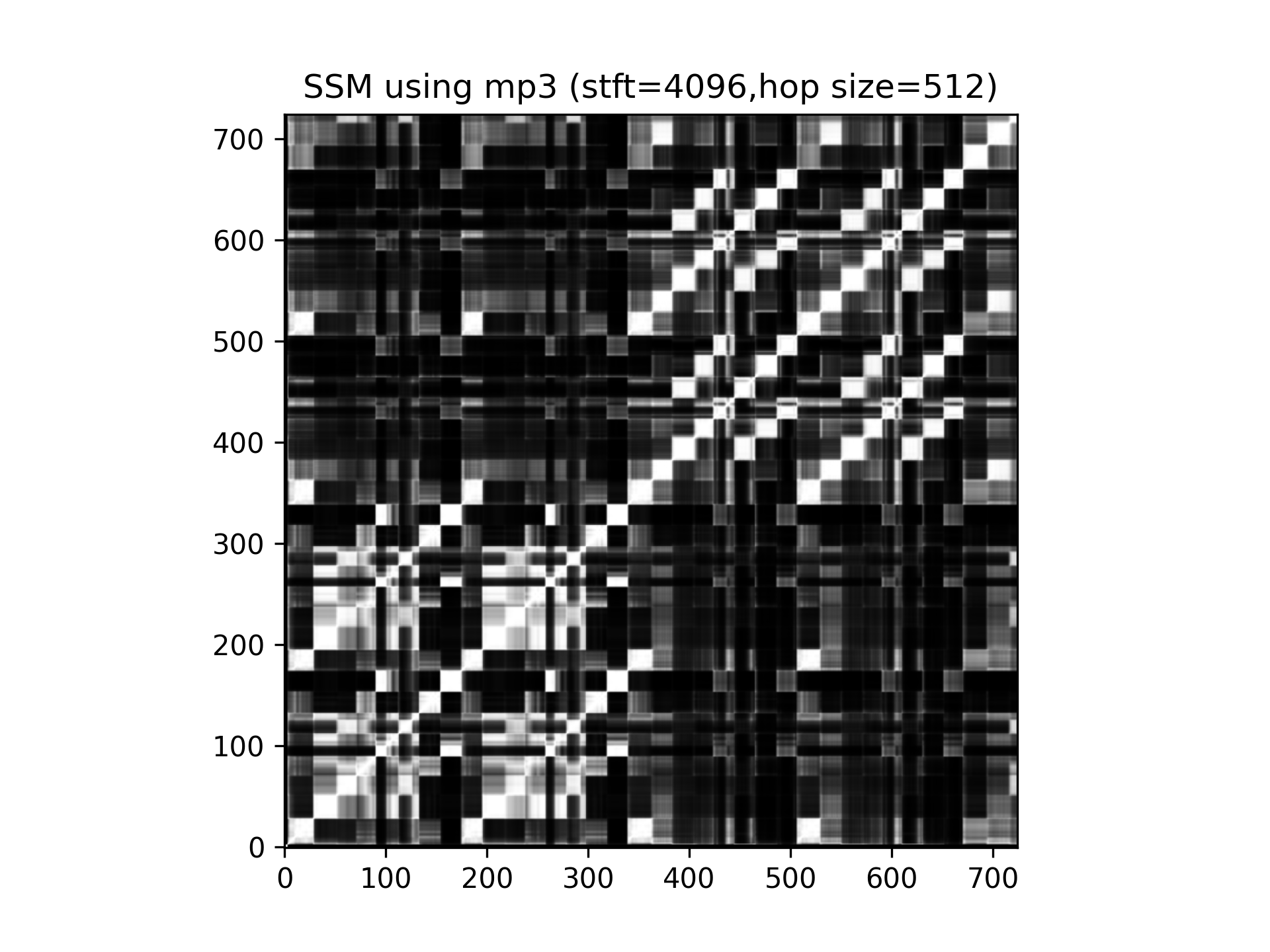
使用audio生成SSM
这里只取前2个bars进行分析:
# %%
import librosa
import matplotlib.pyplot as plt
import numpy as np
from sklearn.metrics.pairwise import cosine_similarity
import time

y, fs = librosa.load('/home/pyAudio/gould_bwv846_first2bars.mp3', sr=44100)

feature = librosa.feature.melspectrogram(y=y, sr=fs, n_fft=4086, hop_length=512, window='blackman')

print(feature.shape)

# %%

ssm = cosine_similarity(np.transpose(feature), np.transpose(feature))
print(ssm.shape)

plt.figure()
plt.imshow(ssm, cmap=plt.cm.gray, origin='lower')
plt.title('SSM using mp3 (stft=4096,hop size=512)')
savePath = '/home/pyAudio/matplotlibFig/' + time.strftime('%Y-%m-%d-%H-%M-%S', time.localtime(time.time()))
plt.savefig(savePath + '.png', dpi=300)
结果如下:
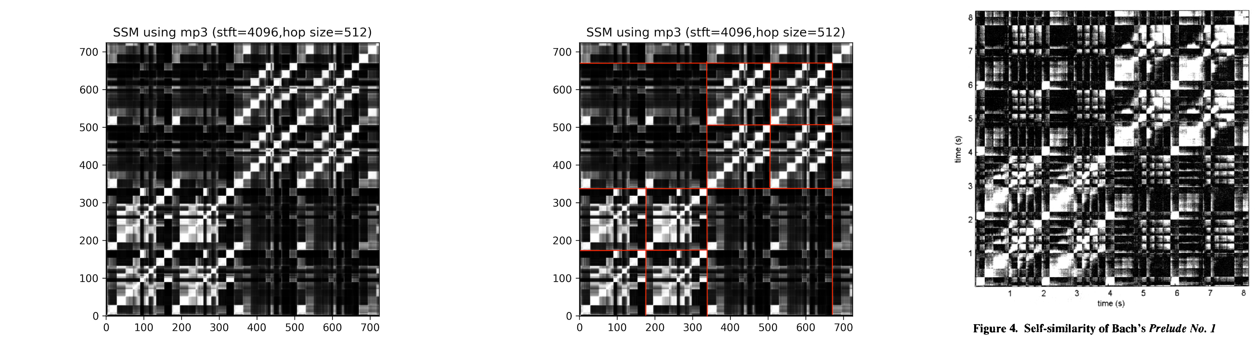
使用基于MIDI获得的audio生成SSM
在第1章的基础上进行了一点修改:改用“质量更高“的音频文件,获得效果更好的SSM图片。但SSM代码的本质仍然是使用librosa.melspectrogram()进行分析,只是使用的audio来自MIDI:
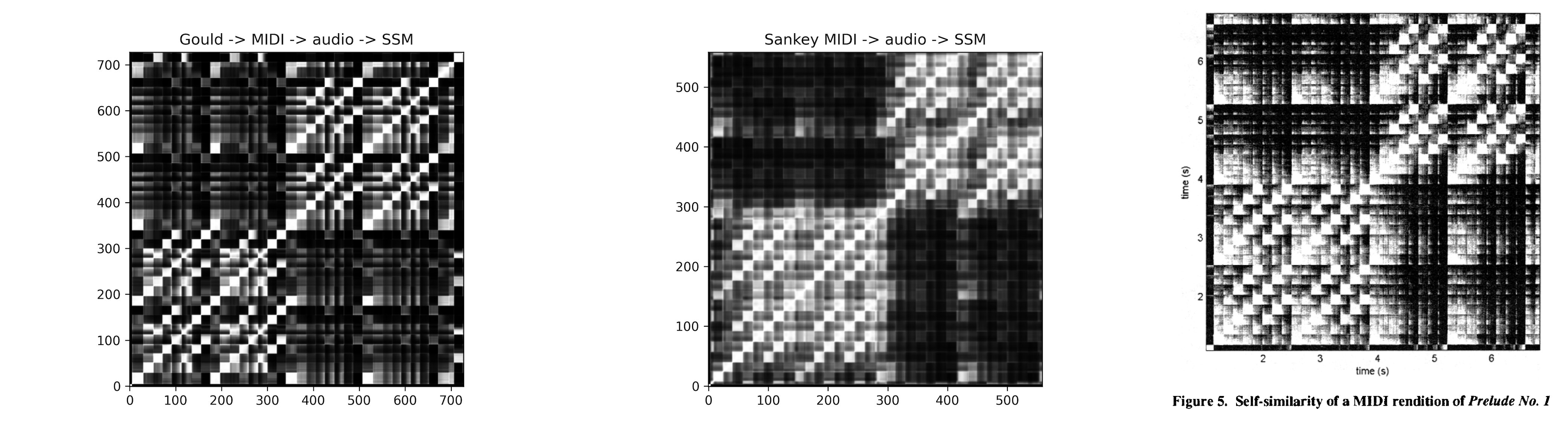
(各种渠道获得的)MIDI -> audio -> melspectrogram -> SSM
使用piano_transcription制作MIDI
第一章中使用了Glenn Gould的作品(audio格式),现在需要把它转换为MIDI格式,然后使用MIDI文件重新制作一次audio。我选择了piano_transcription进行转换,然后使用VLC的convert功能重制了audio,最后对audio进行分析(代码和第1章基本一样,只有读取音频文件的区别,同样只取前2个bars进行分析)。
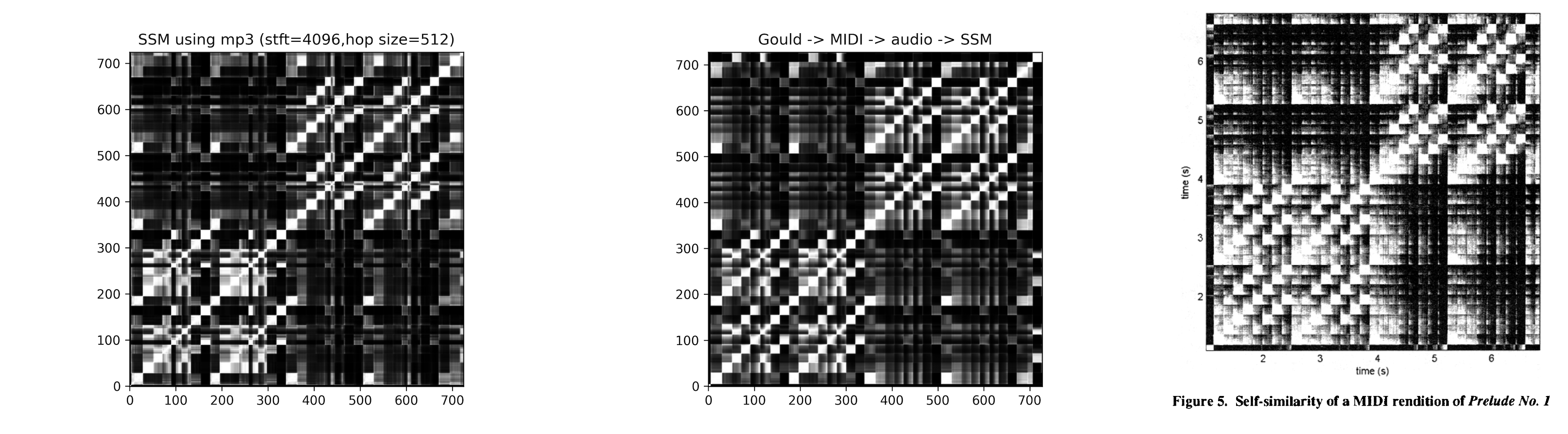
使用其他MIDI文件
从http://www.jsbach.net/midi/midi_johnsankey.html下载了根据John Sankey演奏获得的MIDI文件,按照类似的步骤执行转换与分析,得到结果如下:
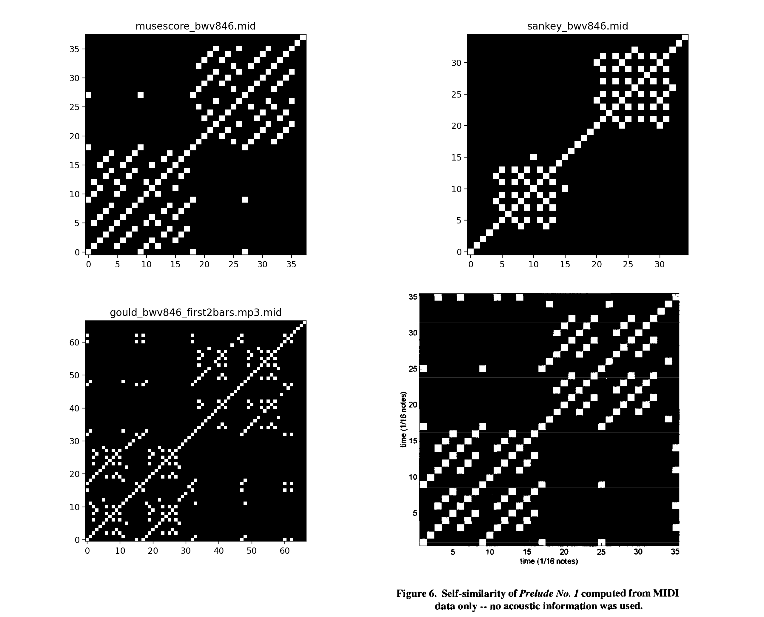
直接对MIDI进行分析生成SSM
代码:
# %%
import pretty_midi
import matplotlib.pyplot as plt
import numpy as np
import time

# midipath = '/home/pyAudio/musescore_bwv846.mid'
# midi_data = pretty_midi.PrettyMIDI(midipath)
# piano_roll = midi_data.get_piano_roll()
# piano_roll = piano_roll[:, 0:int(piano_roll.shape[1] * 2 / 34)]

midipath='/home/pyAudio/sankey_bwv846.mid'
midi_data = pretty_midi.PrettyMIDI(midipath)
piano_roll = midi_data.get_piano_roll()
piano_roll = piano_roll[:, 0:int(piano_roll.shape[1] * 3.3 / 115)]

# midipath='/home/pyAudio/gould_bwv846_first2bars.mp3.mid'
# midi_data = pretty_midi.PrettyMIDI(midipath)
# piano_roll = midi_data.get_piano_roll()

piano_roll[np.where(piano_roll > 0)] = 127
print(piano_roll.shape)

# %%

# remove duplicate 'neighbour columns' in piano_roll

del_lists = []

for i in range(0, piano_roll.shape[1] - 1):
    if (piano_roll[:, i + 1] == piano_roll[:, i]).all():
        del_lists.append(i + 1)

piano_roll = np.delete(piano_roll, del_lists, axis=1)
print(piano_roll.shape)

# %%

ssm = np.zeros((piano_roll.shape[1], piano_roll.shape[1]))

for i in range(0, piano_roll.shape[1]):
    a = piano_roll[:, i]
    for j in range(0, piano_roll.shape[1]):
        b = piano_roll[:, j]
        if (a == b).all():
            ssm[piano_roll.shape[1] - 1 - j, i] = 1

ssm = np.flipud(ssm)
print(ssm.shape)

plt.figure()
plt.imshow(ssm, cmap=plt.cm.gray, origin='lower')
plt.title(midipath.split('/')[-1])
savePath = '/home/pyAudio/matplotlibFig/' + time.strftime('%Y-%m-%d-%H-%M-%S', time.localtime(time.time()))
plt.savefig(savePath + '.png', dpi=200)
在代码的7~19行指定了3种不同的MIDI音源:
1,musescore_bwv846.mid:从musescore.com下载的MIDI文件
2,sankey_bwv846.mid:从jsbach.net下载的MIDI文件
3,gould_bwv846_first2bars.mp3.mid:使用piano_transcription转换Glenn Gould的作品为MIDI文件
代码运行结果如下:
References
[1]. ^ Müller, Meinard. Fundamentals of music processing: Audio, analysis, algorithms, applications. Springer, 2015.
[2]. ^ Foote, Jonathan. "Visualizing music and audio using self-similarity." Proceedings of the seventh ACM international conference on Multimedia (Part 1). 1999.
