 WARNING: This article may be obsolete
This post was published in 2023-08-22. Obviously, expired content is less useful to users if it has already pasted its expiration date.
 This article is categorized as "Garbage" . It should NEVER be appeared in your search engine's results.
Table of Contents
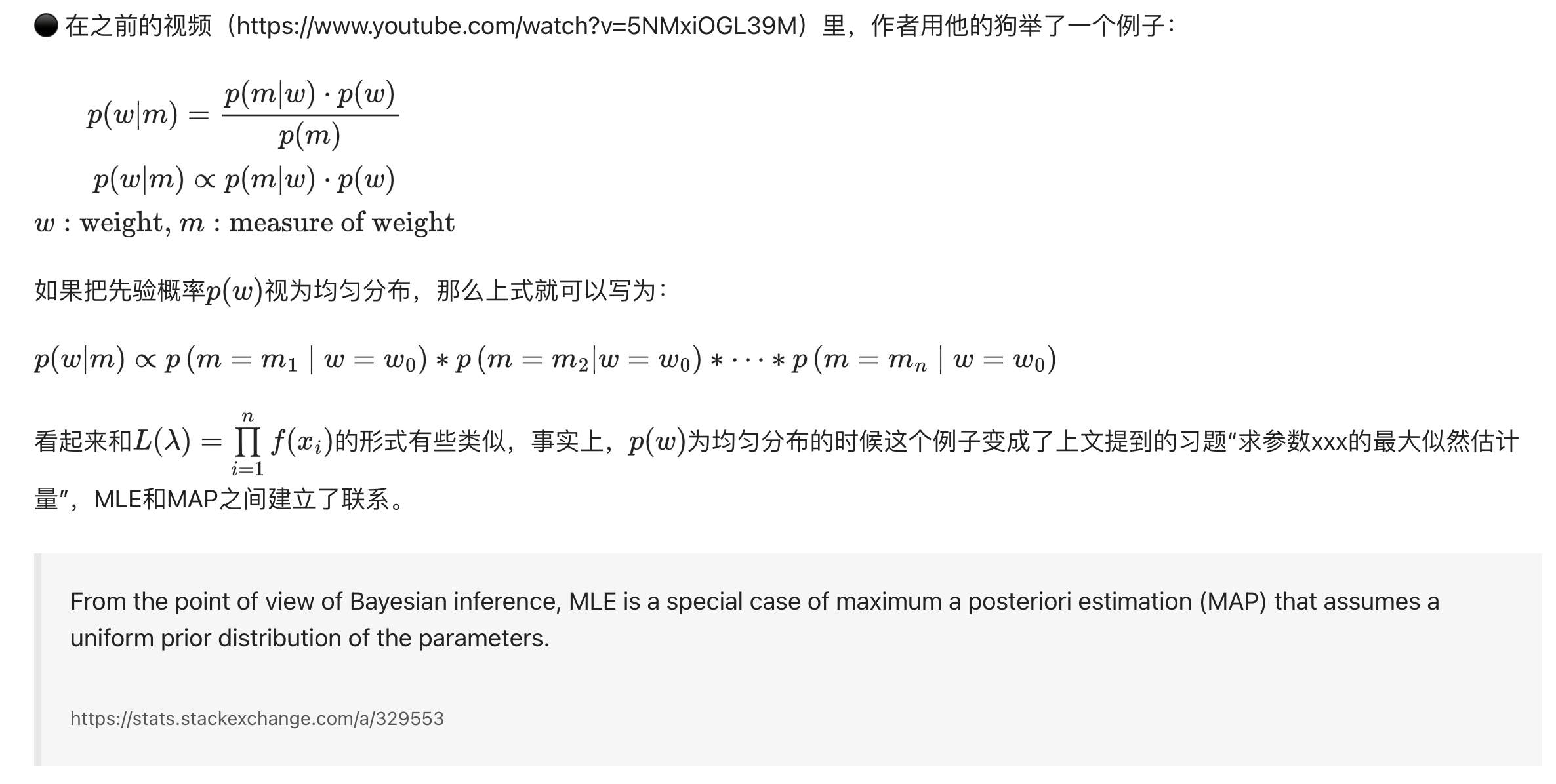
为什么会有这篇笔记?
本笔记写于2023年8月,原因是发现自己时隔一年无法盲背prior/posterior/MLE/MAP的一些概念,尤其是MLE和MAP.
所以本笔记不怎么涉及贝叶斯网络/贝叶斯滤波/卡尔曼滤波 等内容,能重新学会就可以,并不一定需要把所有的笔记列举完毕,因为过去2年写的笔记里和条件概率挂钩的东西有点多,各个角落里都有。更新:甚至不需要专门做一个笔记整理集合。
下面是从零开始回顾这些概念的学习笔记:
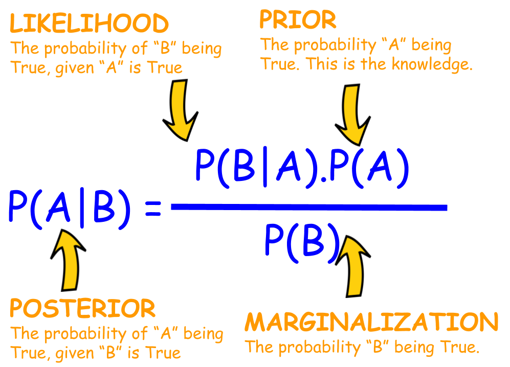
最开始根据惯性记忆写出了这个公式:
[mathjax-d]P(A \mid B)=\frac{P(B \mid A) \cdot P(A)}{P(B)}[/mathjax-d]
知道[mathjax]P(A \mid B)[/mathjax]是posterior,[mathjax]P(A)[/mathjax]是prior,然后剩下的就记不得了,尤其是对[mathjax]P(B \mid A)[/mathjax]和[mathjax]P(B)[/mathjax]解释不清。所以本篇笔记也就是从这里开始的。
重新理解Likelihood,MLE,MAP等概念
[mathjax-d]P(A \mid B)=\frac{P(B \mid A) \cdot P(A)}{P(B)}[/mathjax-d]
通过复习现在知道了[mathjax]P(B \mid A)[/mathjax]是"Likelihood", [mathjax]P(B)[/mathjax]是"Evidence",接下来要完全理解这些概念:
现在一个关键的问题在于如何重新理解Likelihood
先搜集一些wikipedia的严谨定义:
The likelihood function (often simply called the likelihood) is the joint probability of observed data viewed as a function of the parameters of a statistical model.
https://en.wikipedia.org/wiki/Likelihood_function
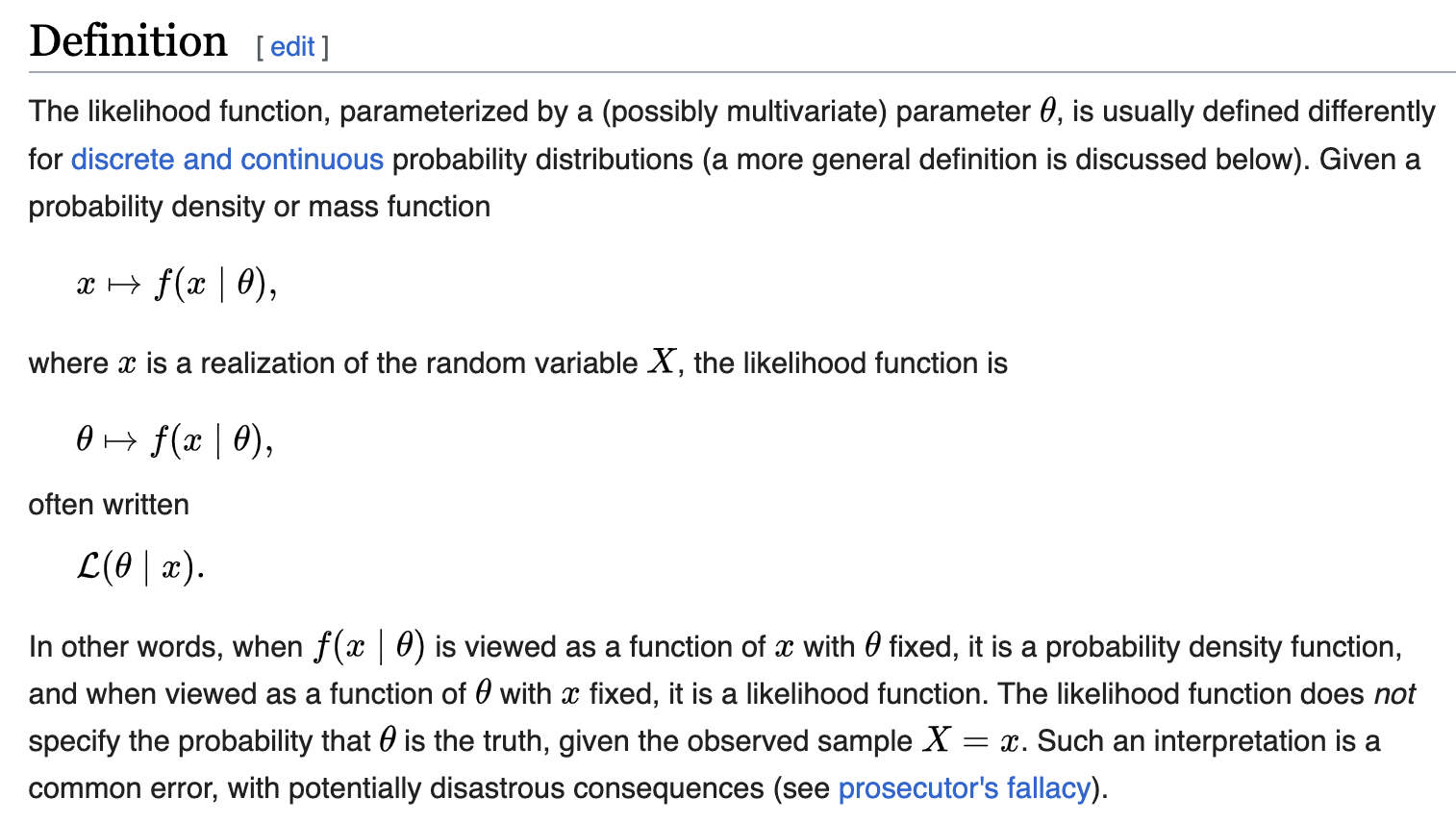
好了,现在开始解释:
一枚正反面均匀的硬币随机扔50次,你认为扔出“正面25,反面25”的可能性有多大?可以用[mathjax]{{50}\choose{25}}(0.5)^{25}(0.5)^{25}[/mathjax]计算出这个概率,得到的结果就是likelihood.
那么,MLE - maximum Likelihood呢?当然就是 argmax(模型) ,也就是说“当这个概率模型长什么样的时候,它最有可能生成这些数据“。
比如硬币的问题:
一个硬币扔了10000次,其中5000次正面,5000次反面,那么我认为它最有可能是什么样子的硬币?我当然会认为它最有可能是一枚正反面均匀的硬币。
那么,MAP - maximize a posteriori(或者写成maximum a posteriori)呢?其实同样是对 模型 的估量(推测这个模型最有可能长什么样),只不过MAP属于贝叶斯学派,他们会先天的给这个模型添加一个prior作为“偏见”,仅此而已!
所以回到贝叶斯的公式:
[mathjax-d]P(A \mid B)=\frac{{\color{red}P(B \mid A)} \cdot P(A)}{P(B)}[/mathjax-d]
整个公式是属于MAP的,而MLE只关心[mathjax]\color{red}P(B \mid A)[/mathjax]这一个东西而已!
接下来会继续建立MLE和MAP的联系:
前面学习MLE的时候已经知道了,MLE的本质就是argmax(模型),那么具体是怎么做的呢?
当然我们学过点估计/矩估计这些:🔗 [2022-08-20 - Truxton's blog] https://truxton2blog.com/2022-08-20/
也学过贝叶斯估计:🔗 [2021-10-22 - Truxton's blog] https://truxton2blog.com/2021-10-22/
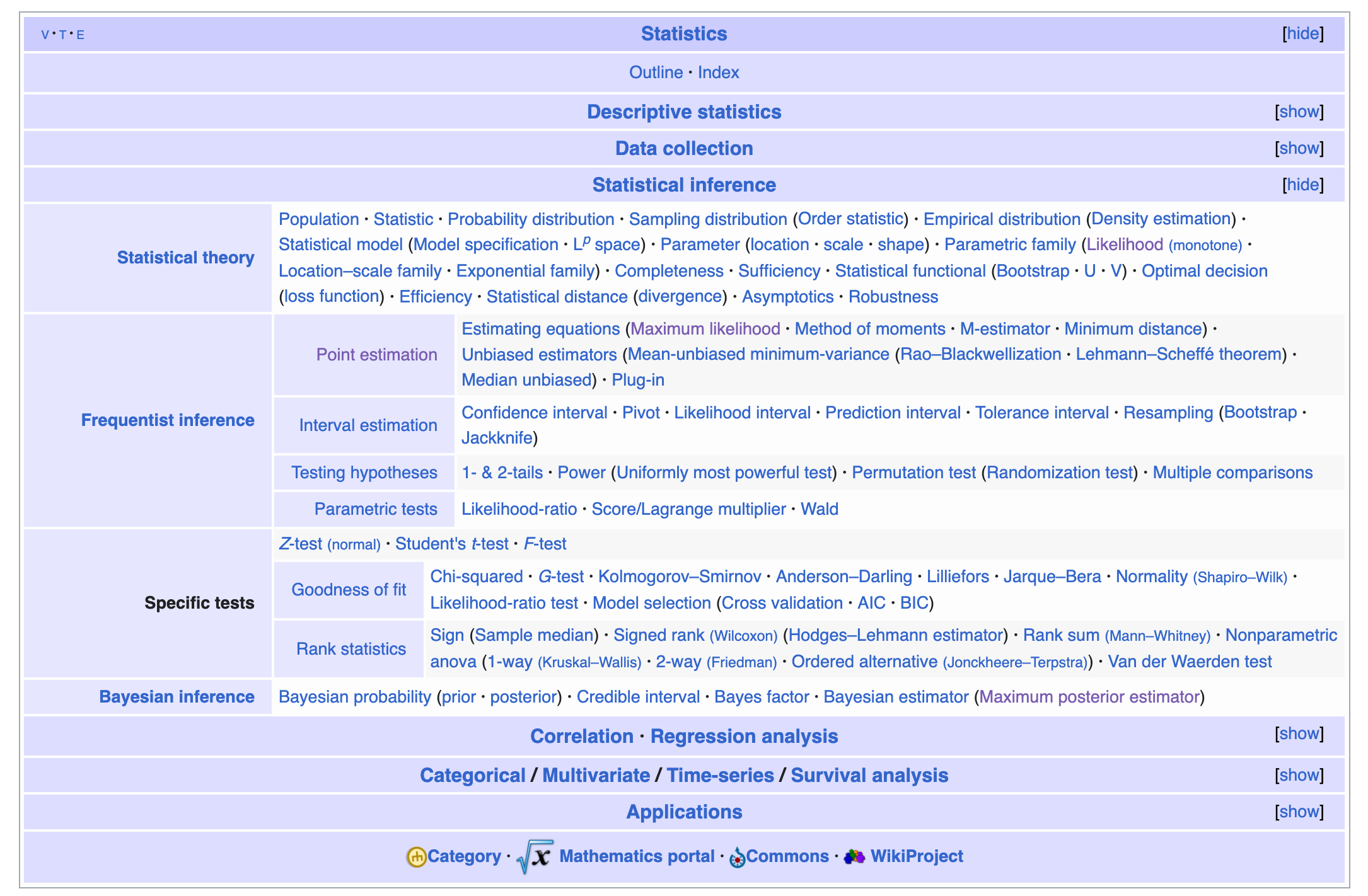
在此之前同时了解一下 频率学派(Frequentist inference)/点估计/MLE/贝叶斯学派(Bayesian inference)/MAP/...的关系:
(作为标注,下面的图中有一些链接的字体颜色不太一样)
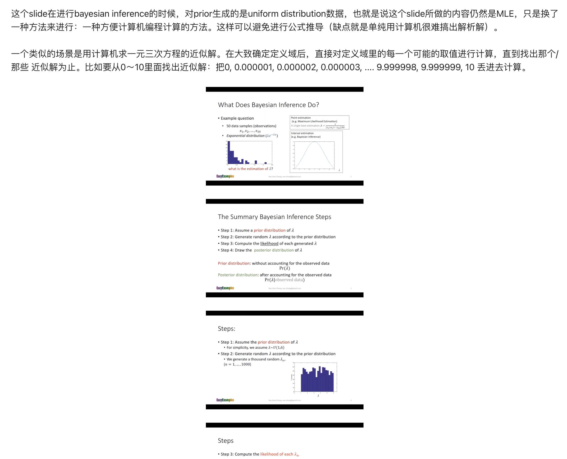
MLE和MAP之间的联系
uniform distribution prior(先验均匀分布)
接下来讨论MLE和MAP之间产生联系的条件:
- prior: uniform distribution,此时MLE=MAP
- observe data -> [mathjax]\infty[/mathjax]
先讨论第1个(prior: uniform distribution),这个东西其实在🔗 [2021-10-22 - Truxton's blog] https://truxton2blog.com/2021-10-22/ 就已经有过相关笔记:
在🔗 [2022-08-20 - Truxton's blog] https://truxton2blog.com/2022-08-20/ 也有提到:

观测数据趋于无限
再来讨论第2个:observe data -> [mathjax]\infty[/mathjax]
严谨的证明暂时不会,相关讨论可以后续有机会看:🔗 [Maximum likelihood equivalent to maximum a posterior estimation - Cross Validated] https://stats.stackexchange.com/questions/52395/maximum-likelihood-equivalent-to-maximum-a-posterior-estimation
先想象一些东西:
相比于政府发行的巨量硬币(正常硬币),地球上很难找到一枚明显正反面不均匀的硬币,所以贝叶斯学派有了一个相当强硬的prior,认为P(硬币随机扔出正面)= 0.5 . 但现在我们给贝叶斯学派送出了一组观测数据,
数据结果表明:扔了10次,4次正面,此时贝叶斯学派认为这只是观测数据太少,这枚硬币大概率还是正反面均匀的。
又来了一组数据:扔了100次,40次正面,此时贝叶斯学派的计算结果会继续靠近0.4(认为这枚硬币确实大概率是正反面不均匀的)
又来了一组数据:扔了100000次,40000次正面,此时贝叶斯学派的计算结果会非常非常靠近0.4
又来了一组数据:扔了10000000次,4000000次正面,此时贝叶斯学派的计算结果会非常非常非常靠近0.4
....
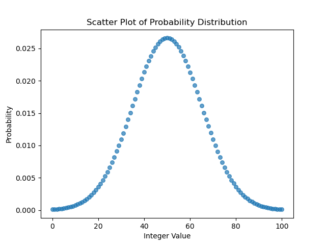
写个程序模拟一下这个硬币实验,其中贝叶斯学派的人认为硬币投出正面的prior是[mathjax]\mu=0.5[/mathjax]的正态分布(联动一下🔗 [2025-05-26 - Truxton's blog] https://truxton2blog.com/2025-05-26/ 的代码,中心极限定理-二项分布,抛硬币计为正面=1反面=0,sum(X)就是统计抛出正面的次数,接近正态分布)
假设投出了这些结果:
5次-2正
10次-4正
50次-20正
500次-200正
代码是草稿,注意有很多问题:
- 生成normal distribution prior的代码是chatgpt写的,暂时懒得改进了(调了好几次才调好,最后用的还是我的思路,chatgpt似乎变笨了)
- 就算是调好的chatgpt代码仍然一堆问题:2024-02-14我又发现了2个问题,并整理了一篇笔记:🔗 [2024-02-14 有关numpy整数处理的一些问题 - Truxton's blog] https://truxton2blog.com/2024-02-14-numpy-integer-handling-issue/
- 画图看个大概就行,坐标轴没有调的
from math import comb
import matplotlib.pyplot as plt
import numpy as np
import random

result_group = []
for total in (5, 10, 50, 500):
    prob = []
    for p in np.arange(0, 1.01, 0.01):
        front = int(total * 0.4)
        back = total - front
        prob.append(comb(total, front) * np.power(p, front) * np.power((1 - p), back))
    result_group.append(prob)

plt.figure()
plt.plot(result_group[0], color="black", label="5")
plt.plot(result_group[1], color="green", label="10")
plt.plot(result_group[2], color="blue", label="50")
plt.plot(result_group[3], color="red", label="500")
plt.legend()
plt.savefig('MLE.png')

########################################################
# begin stupid chatgpt code
# 2024-02-14 我发现原本代码里的np.clip()有问题,进行了修改,同时增大了num_values,目的是让prior更精确
# 2024-02-14 我发现原本代码里的np.random.normal(mean, std_deviation, num_values).astype(int)有问题,会导致生成的0比1多(因为-0.x也被算成了0)

mean = 50
std_deviation = 15
num_values = 100000000

raw_integer_values = np.rint(np.random.normal(mean, std_deviation, num_values)).astype(int)

filtered_integer_values = raw_integer_values[(raw_integer_values >= 0) & (raw_integer_values <= 100)]

# Count the occurrences of each integer value
counter = np.bincount(filtered_integer_values, minlength=101)

# Normalize the counter array to get probabilities
probabilities = counter / np.sum(counter)

# Generate x values for the scatter plot (integer values)
x_values = np.arange(0, 101)

# Create a scatter plot
plt.figure()
plt.scatter(x_values, probabilities, marker='o', s=30, alpha=0.7)
plt.xlabel("Integer Value")
plt.ylabel("Probability")
plt.title("Scatter Plot of Probability Distribution")
plt.savefig('prior.png')

# end stupid chatgpt code
########################################################


posterior_group = []
for group in result_group:
    if (len(group) != len(probabilities)):
        print('check your code')
        exit(1)
    temp = []
    for i in range(0, len(group)):
        temp.append(group[i] * probabilities[i])
    posterior_group.append(temp)

plt.figure()
plt.plot(posterior_group[0], color="black", label="5")
plt.plot(posterior_group[1], color="green", label="10")
plt.plot(posterior_group[2], color="blue", label="50")
plt.plot(posterior_group[3], color="red", label="500")
plt.legend()
plt.savefig('MAP.png')
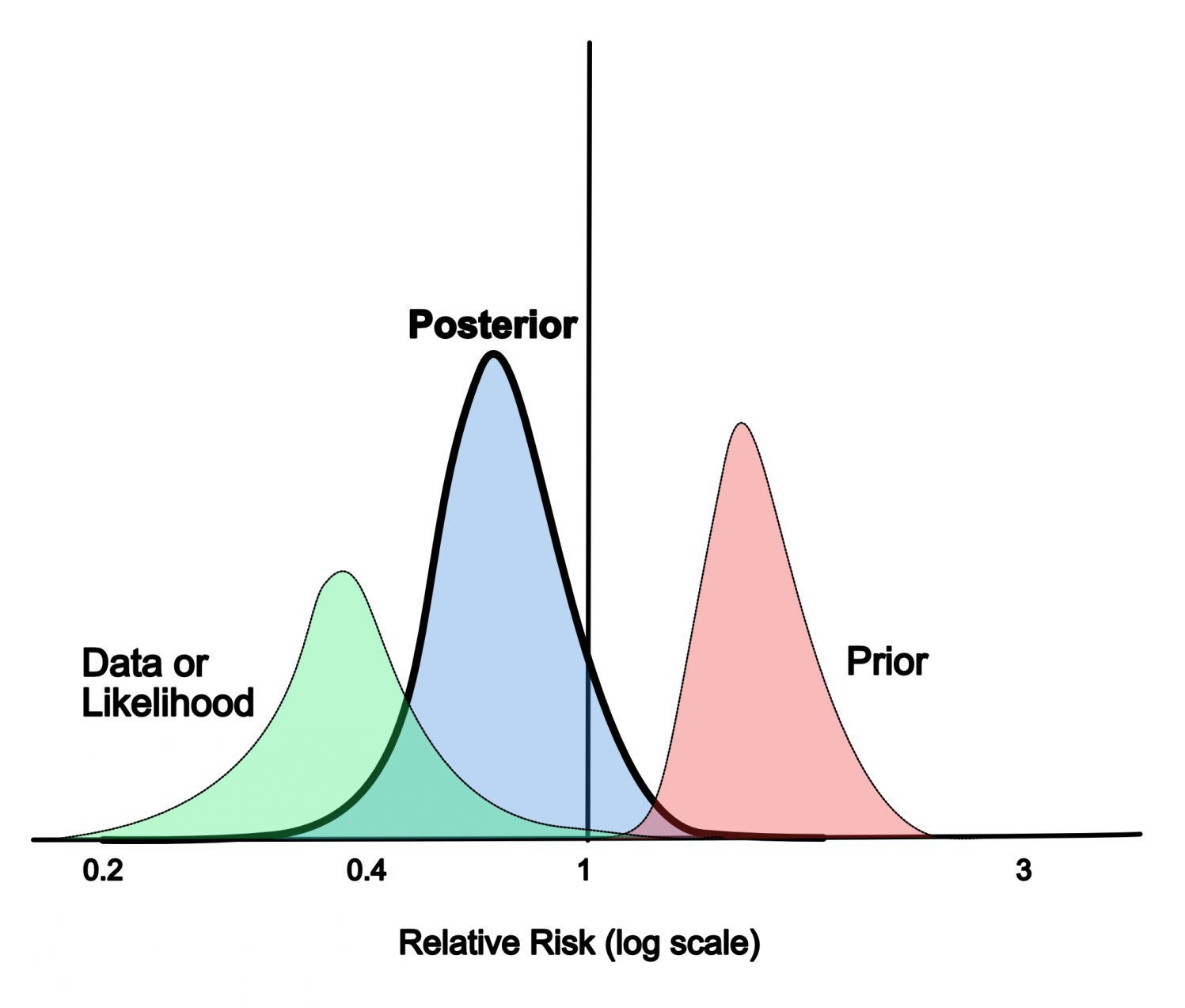
结果:
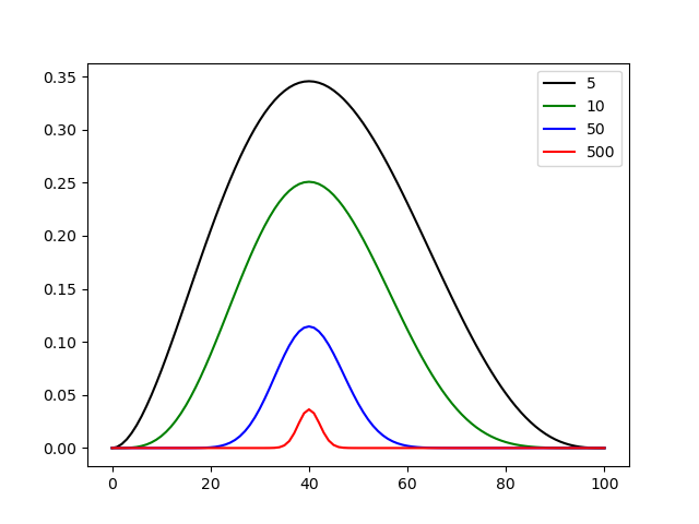
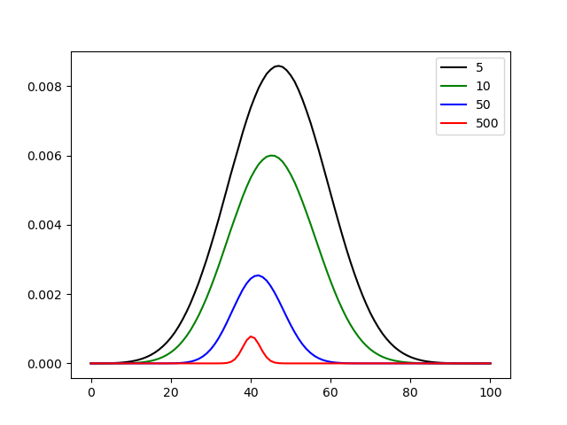
从MAP.png可以看出,随着数据的不断增多,贝叶斯学派对这枚硬币的看法会不断接近40(代表P=0.4,懒得改坐标轴代码了)
注意,MLE和MAP的纵坐标放在一起对比没什么意义,对模型的估计要的是argmax(模型),也就是说模型分布的中心趋向于哪里就估计哪里。
