 WARNING: This article may be obsolete
This post was published in 2022-06-03. Obviously, expired content is less useful to users if it has already pasted its expiration date.
 This article is categorized as "Garbage" . It should NEVER be appeared in your search engine's results.
Table of Contents
重新复习傅里叶变换
重新复习🔗 [ASPMA课程大纲复习(2021-06初版) - Truxton's blog] https://truxton2blog.com/aspma-syllabus-review/,这篇笔记还是不够入门,现在记录一些更入门的东西。
读取音频文件,FFT简单分析(scipy)
呃...可以先参考这篇写过的文章:🔗 [ASPMA补充材料(1):DFT、FFT、Minimize energy spread in DFT of sinusoids的python3实现 - Truxton's blog] https://truxton2blog.com/aspma-syllabus-review-supplement-1-dft-fft-energy-spread/
回忆这个问题:
有关Amplitude scaling:
(先空着)
代码1:单纯的读
一段毫无修饰和变换的代码:
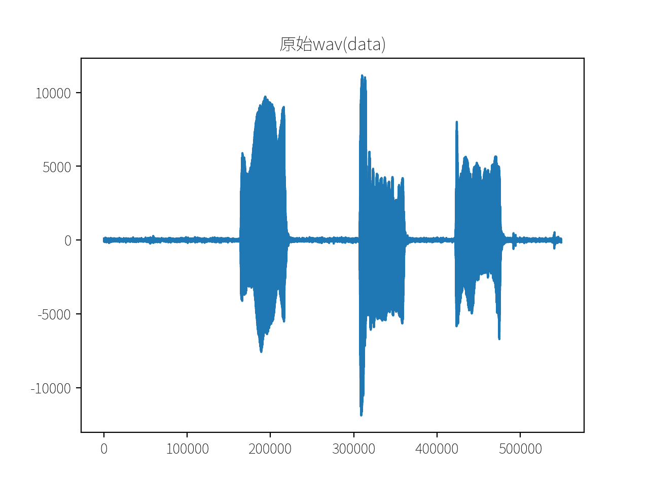
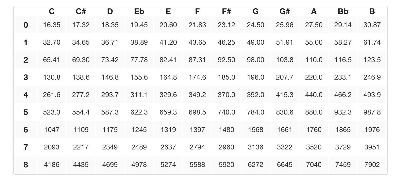
注: 1.wav 是使用高音竖笛吹出来的C, C#, D
from scipy.io import wavfile
from scipy.fftpack import fft
import numpy as np
import matplotlib.pyplot as plt
import matplotlib as mpl
# dpi和中文字体
mpl.rcParams['figure.dpi'] = 200
plt.rcParams['font.sans-serif'] = ['Source Han Sans']
plt.rcParams['axes.unicode_minus'] = False
fs, data = wavfile.read('1.wav')
print(fs)
plt.figure()
plt.plot(data)
plt.title('原始wav')
plt.savefig('0.png')
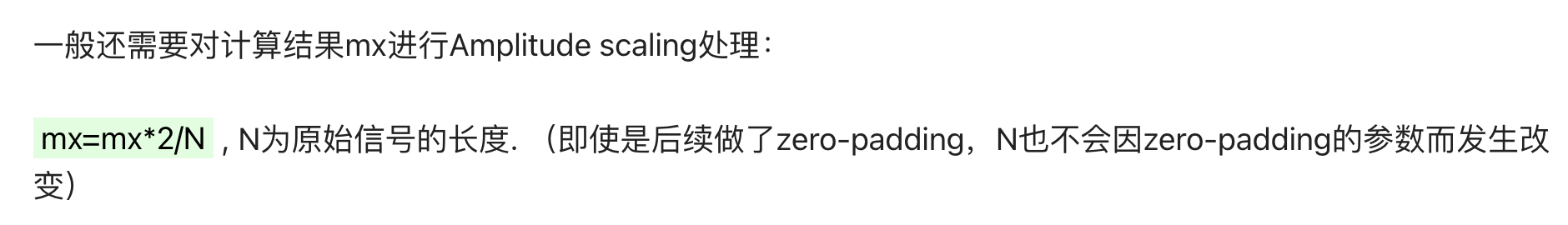
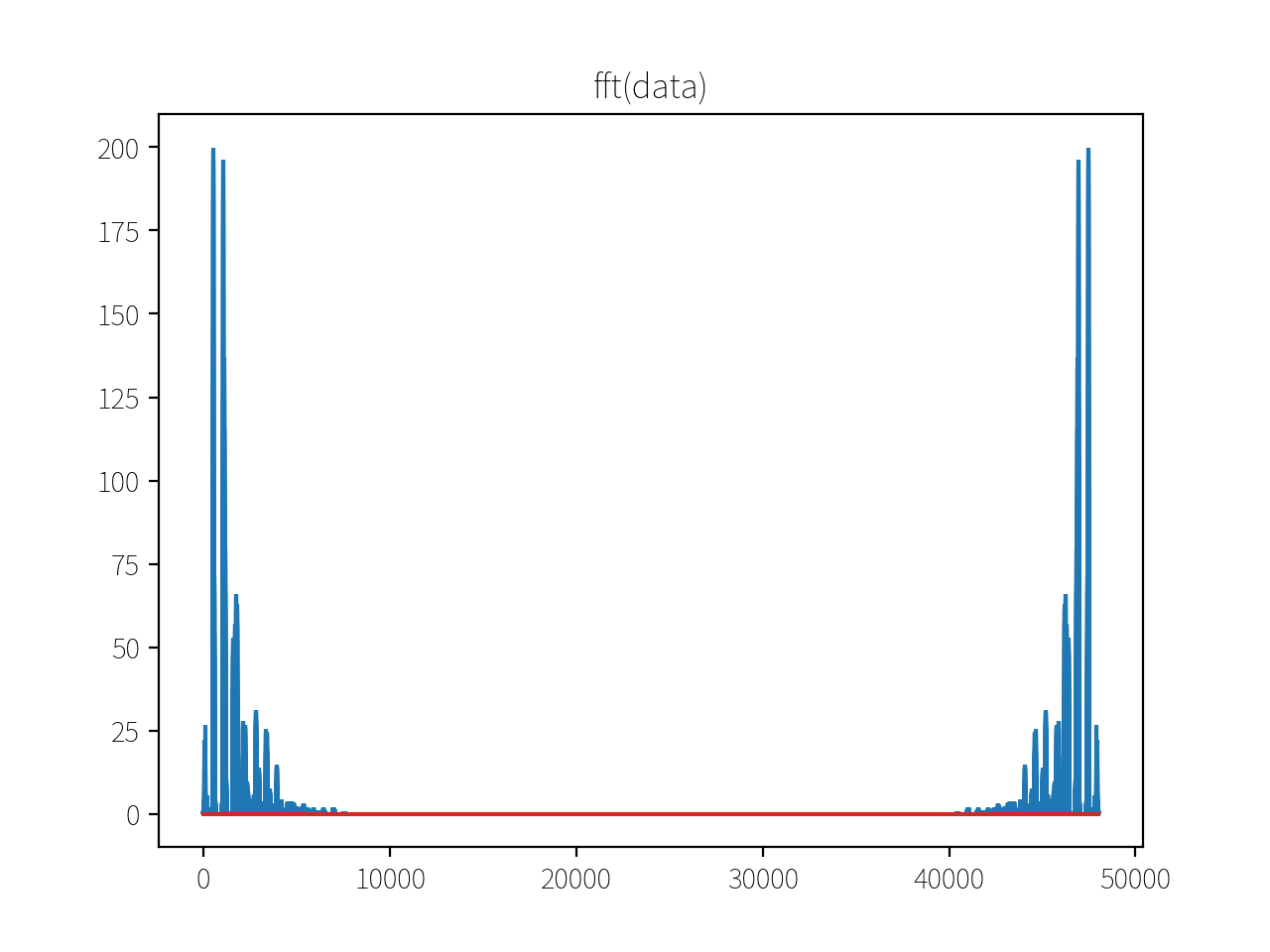
mx = np.abs(fft(data))
plt.figure()
plt.stem(data)
plt.title('fft(data)')
plt.savefig('1.png')

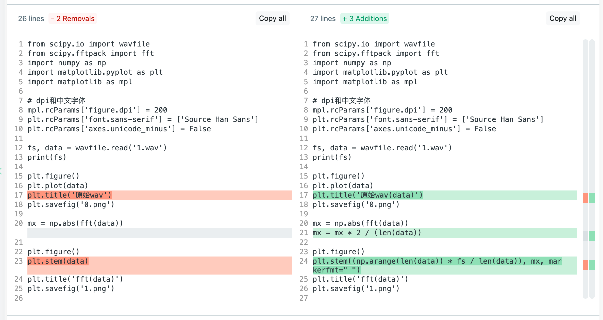
代码2:缩放、变换、frequency-bins转换为frequency
然后修改一下:
from scipy.io import wavfile
from scipy.fftpack import fft
import numpy as np
import matplotlib.pyplot as plt
import matplotlib as mpl

# dpi和中文字体
mpl.rcParams['figure.dpi'] = 200
plt.rcParams['font.sans-serif'] = ['Source Han Sans']
plt.rcParams['axes.unicode_minus'] = False

fs, data = wavfile.read('1.wav')
print(fs)

plt.figure()
plt.plot(data)
plt.title('原始wav(data)')
plt.savefig('0.png')

mx = np.abs(fft(data))
mx = mx * 2 / (len(data))

plt.figure()
plt.stem((np.arange(len(data)) * fs / len(data)), mx, markerfmt=" ")
plt.title('fft(data)')
plt.savefig('1.png')
由于FFT的对称性,现在观察fft(data)的0~1000Hz范围(因为这是高音竖笛,参考这张图片):
(鸽了)
包络线
最开始出现在ASPMA课程的这个地方:
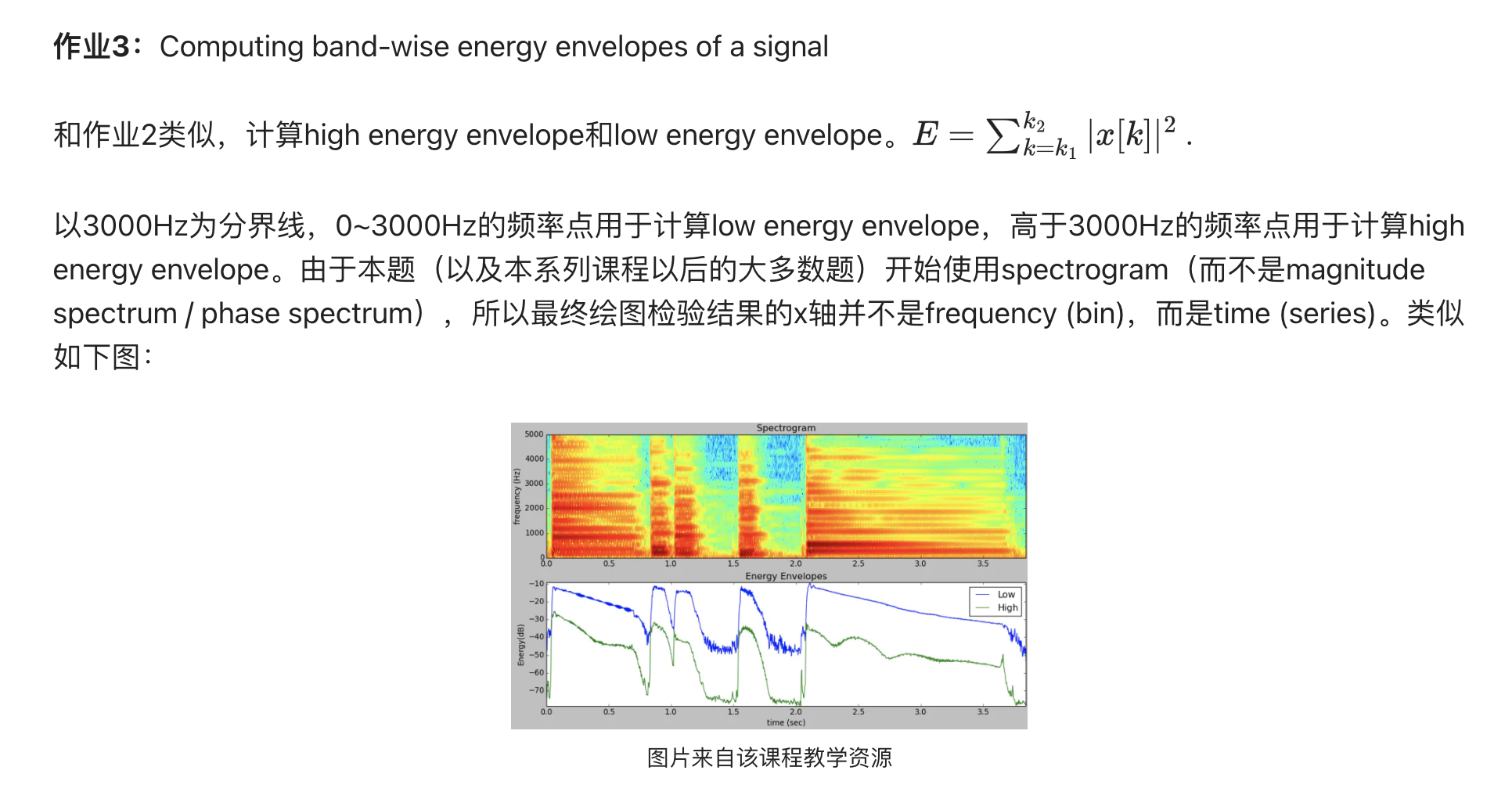
在A4Part3.py里,对envelope作业的描述:
折叠
"""
A4-Part-3: Computing band-wise energy envelopes of a signal
Write a function that computes band-wise energy envelopes of a given audio signal by using the STFT.
Consider two frequency bands for this question, low and high. The low frequency band is the set of
all the frequencies between 0 and 3000 Hz and the high frequency band is the set of all the
frequencies between 3000 and 10000 Hz (excluding the boundary frequencies in both the cases).
At a given frame, the value of the energy envelope of a band can be computed as the sum of squared
values of all the frequency coefficients in that band. Compute the energy envelopes in decibels.
Refer to "A4-STFT.pdf" document for further details on computing bandwise energy.
The input arguments to the function are the wav file name including the path (inputFile), window
type (window), window length (M), FFT size (N) and hop size (H). The function should return a numpy
array with two columns, where the first column is the energy envelope of the low frequency band and
the second column is that of the high frequency band.
Use stft.stftAnal() to obtain the STFT magnitude spectrum for all the audio frames. Then compute two
energy values for each frequency band specified. While calculating frequency bins for each frequency
band, consider only the bins that are within the specified frequency range. For example, for the low
frequency band consider only the bins with frequency > 0 Hz and < 3000 Hz (you can use np.where() to
find those bin indexes). This way we also remove the DC offset in the signal in energy envelope
computation. The frequency corresponding to the bin index k can be computed as k*fs/N, where fs is
the sampling rate of the signal.
To get a better understanding of the energy envelope and its characteristics you can plot the envelopes
together with the spectrogram of the signal. You can use matplotlib plotting library for this purpose.
To visualize the spectrogram of a signal, a good option is to use colormesh. You can reuse the code in
sms-tools/lectures/4-STFT/plots-code/spectrogram.py. Either overlay the envelopes on the spectrogram
or plot them in a different subplot. Make sure you use the same range of the x-axis for both the
spectrogram and the energy envelopes.
NOTE: Running these test cases might take a few seconds depending on your hardware.
Test case 1: Use piano.wav file with window = 'blackman', M = 513, N = 1024 and H = 128 as input.
The bin indexes of the low frequency band span from 1 to 69 (69 samples) and of the high frequency
band span from 70 to 232 (163 samples). To numerically compare your output, use loadTestCases.py
script to obtain the expected output.
Test case 2: Use piano.wav file with window = 'blackman', M = 2047, N = 4096 and H = 128 as input.
The bin indexes of the low frequency band span from 1 to 278 (278 samples) and of the high frequency
band span from 279 to 928 (650 samples). To numerically compare your output, use loadTestCases.py
script to obtain the expected output.
Test case 3: Use sax-phrase-short.wav file with window = 'hamming', M = 513, N = 2048 and H = 256 as
input. The bin indexes of the low frequency band span from 1 to 139 (139 samples) and of the high
frequency band span from 140 to 464 (325 samples). To numerically compare your output, use
loadTestCases.py script to obtain the expected output.
In addition to comparing results with the expected output, you can also plot your output for these
test cases.You can clearly notice the sharp attacks and decay of the piano notes for test case 1
(See figure in the accompanying pdf). You can compare this with the output from test case 2 that
uses a larger window. You can infer the influence of window size on sharpness of the note attacks
and discuss it on the forums.
"""
更多参考资料:
🔗 [Envelope (waves) - Wikipedia] https://en.wikipedia.org/wiki/Envelope_(waves)
🔗 [现代语音信号处理笔记 (七) - Pelhans 的博客] http://pelhans.com/2018/07/09/speeh_process_note7/
